How to combine columns in exale

When working in the program, Excel sometimes comes to combine two or more columns. Some users do not know how to do it. Others are familiar only with the simplest options. We will discuss all possible ways to combine these elements, because in each individual case rationally use various options.

Combine Procedure

All ways to combine columns can be divided into two large groups: use formatting and use of functions. The formatting procedure is more simple, but some problems of merging columns can be solved only by using a special function. Consider all the options in more detail and define, in what specific cases it is better to apply a certain method.

Method 1: Combine using the context menu

The most common way to combine columns is to use the context menu tools.

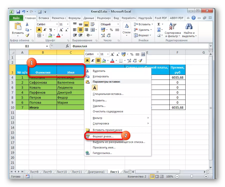
1. We highlight the first range of the cells of the speakers that we want to combine. Click on the dedicated elements with the right mouse button. The context menu opens. Select it in it "Cell format ...".



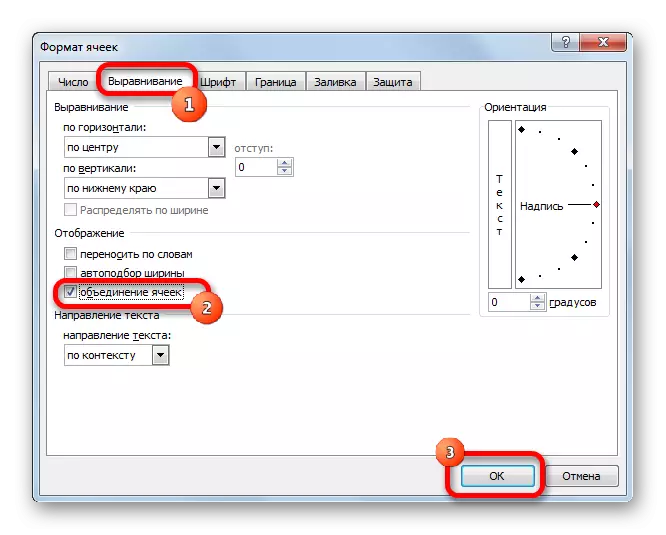
2. Cell formatting window opens. Go to the "Alignment" tab. In the settings group "Display" near the "Customized Combining" parameter, we put a tick. After that, click on the "OK" button.



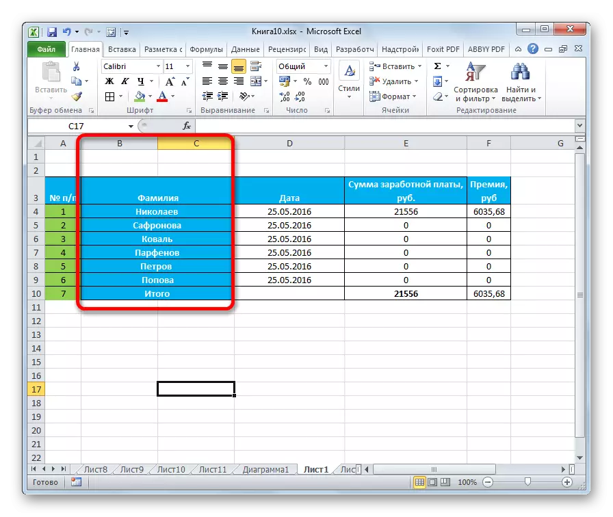
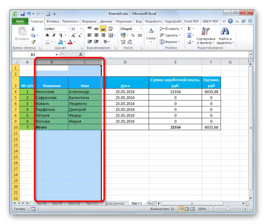
3. As you can see, we combined only the upper cells of the table. We need to combine all cells of the two columns line. Select the combined cell. Being in the "Home" tab on the tape click on the "sample format" button. This button has a brush form and is located in the "Exchange Buffer" toolbar. After that, simply allocate the rest of the remaining area, within which you need to combine columns.



4. After formatting according to the sample, the columns of the table will be combined into one.

Attention! If the data combined in the combined cells, only the information that is located in the first to the left column of the selected interval will be saved. All other data will be destroyed. Therefore, with a rare exception, this method is recommended to be used to work with empty cells or with speakers with low-value data.

Method 2: Combine using the tape button

Also combining columns can be carried out using a tape button. In this way, it is convenient to use if you want to combine not just columns of a separate table, but a sheet as a whole.

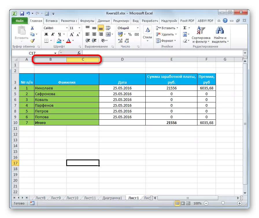
1. In order to combine columns on a sheet completely, they need to highlight them first. We become on the horizontal panel of Excel coordinates, in which the names of the columns with the letters of the Latin alphabet are recorded. Push the left coppe of the mouse and highlight the columns that we want to combine.



2. Go to the "Home" tab, if at the moment we are in another tab. Click on the pictogram in the form of a triangle, the edge of the directional down, to the right of the "Combine and Place in the Center" button, which is located on the tape in the Alignment Tool Block. The menu opens. Choose in it the item "Combine by lines".

After these actions, the allocated columns of the entire sheet will be combined. When using this method, as in the previous embodiment, all data, except those that were in the union in the extreme left column, will be lost.

Method 3: Combine using function

At the same time, it is possible to combine columns without data loss. The implementation of this procedure is much more complicated by the first method. It is carried out using the Capture function.

1. Select any cell in an empty column on the Excel sheet. In order to call the functions wizard, click on the "Insert function" button, located near the formula row.



2. A window opens with a list of various functions. We need among them to find the name "Capture". After you find, select this item and click on the "OK" button.



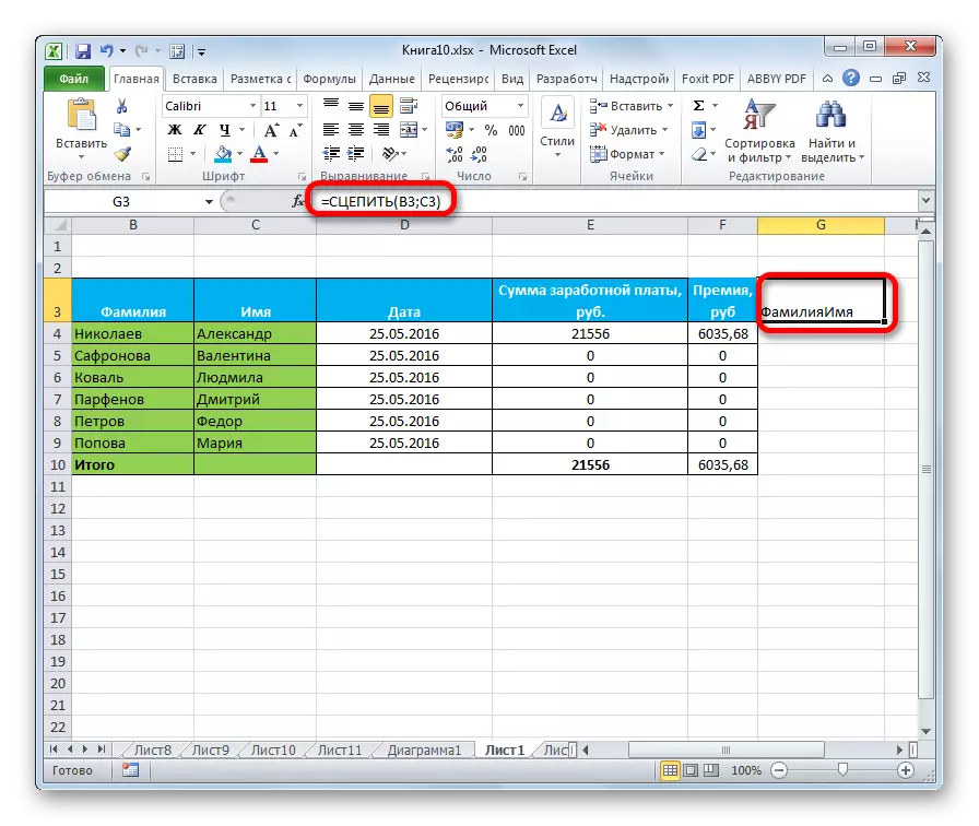
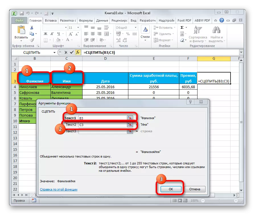
3. After that, the arguments of the argument window opens. Its arguments are cell addresses, the contents of which need to be combined. In the field "Text1", "Text2", etc. We need to make addresses of the cells of the highest row of united columns. You can do it by entering the addresses manually. But it is much more convenient to put the cursor in the field of the corresponding argument, and then select the cell to be associated. In the same way, we actually act with other cells of the first line of the combined columns. After the coordinates appeared in the "Test1" fields, "Text2", etc., press the "OK" button.



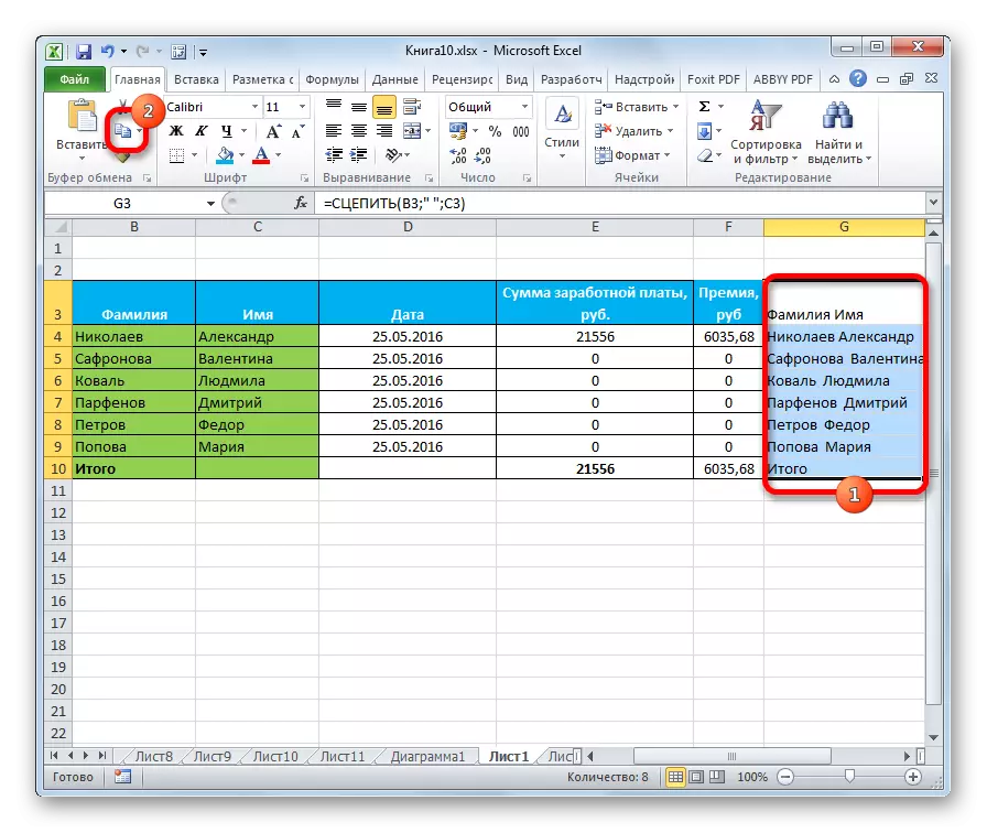
4. In the cell, which displays the result of the processing of values ​​function, the combined data of the first line of the glued columns appeared. But, as we see, the words in the cell merged with the result, there is no space between them.

   

   In order to disconnect them in the formula row after point with a comma between the coordinates of the cells, we insert the following characters:

   " ";

   At the same time, between the two characters in these additional symbols, we put the gap. If we talk about a specific example, then in our case the record:

   = Catch (B3; C3)

   It was changed to the following:

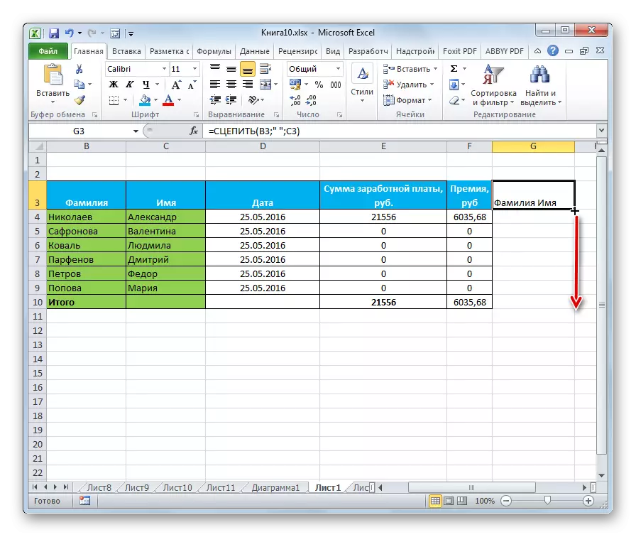
   = Catch (B3; ""; C3)

   As we see, there is a space between the words, and they are no longer merging. If you wish, along with a space, you can put a comma or any other separator.



5. But, while we see the result only for one line. To obtain the combined value of the columns and in other cells, we need to copy the function to thread the bottom range. To do this, set the cursor to the lower right corner of the cell containing the formula. A marker of filling in the form of a cross appears. Click the left mouse button and stretch it down to the end of the table.



6. As we can see, the formula is copied to the range below, and the corresponding results were displayed in the cells. But we just made values ​​in a separate column. Now you need to combine the initial cells and return the data to the original location. If you simply combine or delete the source columns, then the formula to catch will be broken, and we still lose the data. Therefore, we will do a little differently. Select a column with a combined result. In the Home tab, click on the "Copy" button, placed on the tape in the "Exchange Buffer" toolbar. As an alternative action, you can download the CTRL + C keyboard after selecting the column.



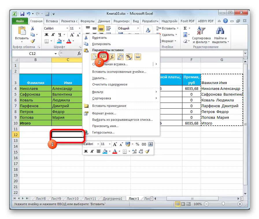
7. Install the cursor on any empty sheet area. Click right mouse button. In the context menu that appears in the Insert Settings block, select the "Value" item.



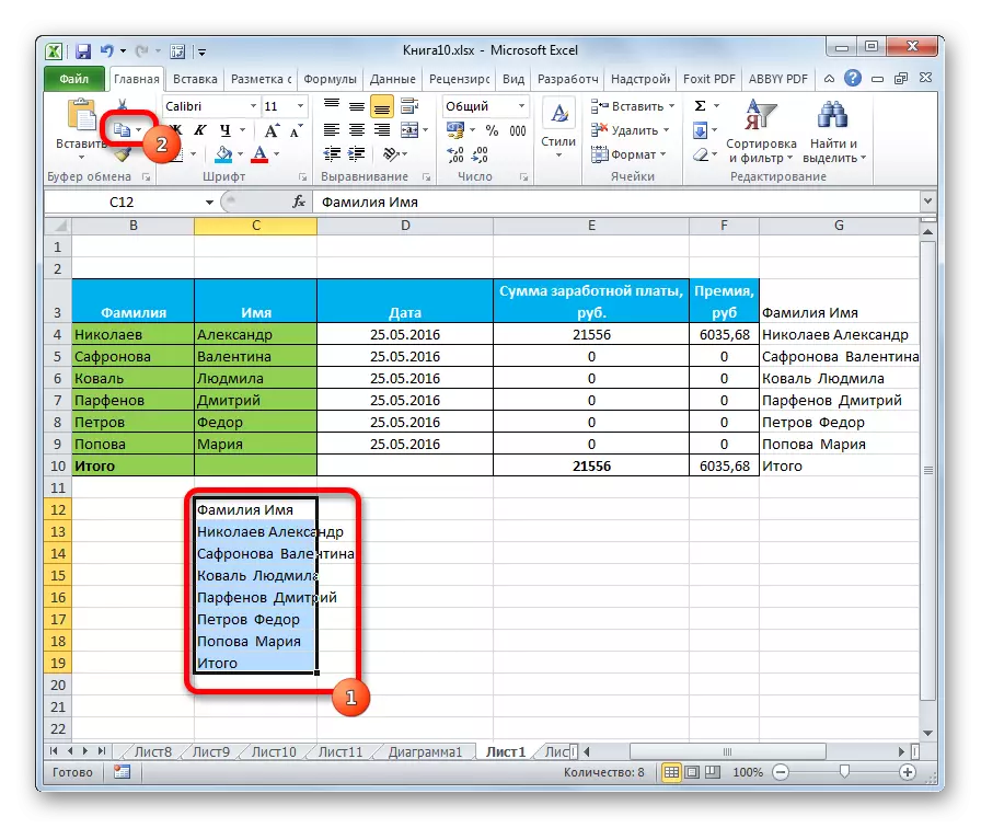
8. We have saved the values ​​of the combined column, and they no longer depend on the formula. Once again copy the data, but already from the new place of their placement.



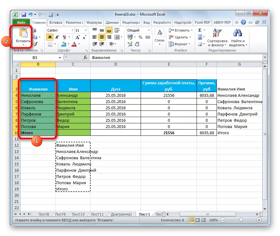
9. We highlight the first column of the initial range, which will need to be combined with other speakers. We click on the "Paste" button posted on the Home tab in the Exchange Buffer toolbu. You can, instead of the last steps, press the keyboard shortcut Ctrl + V keys.



10. Select the initial columns that should be combined. In the Home tab, in the "Alignment" toolbar, you already open a familiar to us by the previous method of the menu and choose the "Combine by line" item in it.



11. After that, a window with an informational message on data loss will appear several times. Press the "OK" button each time.



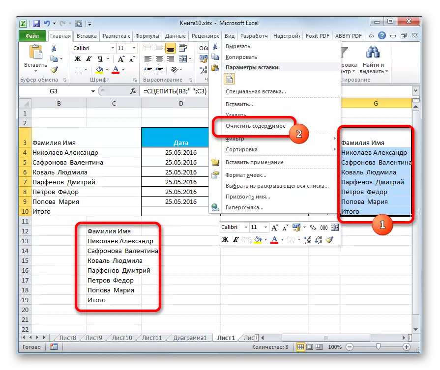
12. As you can see, the data is finally combined in the same column in the place in which it was originally required. Now you need to clean the sheet from transit data. We have two areas: column with formulas and column with copied values. We allocate alternately first and second range. Right-click on the selected area. In the context menu, select the "Clean Content" item.



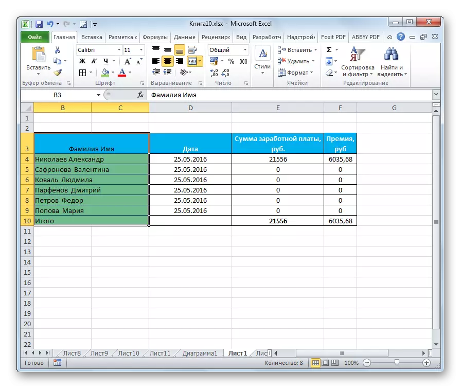
13. After we got rid of transit data, format the combined column at their discretion, as due to our manipulations, its format was reset. It all depends on the target of the specific table and remains at the discretion of the user.

On this procedure, the combination of columns without data loss can be considered over. Of course, this method is much more complicated by previous options, but in some cases it is indispensable.

Lesson: Wizard Functions in Excel

As you can see, there are several ways to combine columns in Excel. You can use any of them, but under certain circumstances, you should give preference to a specific option.

So, most users prefer to use combining through the context menu, as the most intuitive. If you need to make the fusion of columns not only in the table, but also throughout the sheet, then it will be formatted through the menu item on the rinse ribbon. If you need to combine without loss of data, then you can cope with this task only by using the Capture function. Although if the data saving tasks are not put, and even more so, if the united cells are empty, then it is not recommended to use this option. This is due to the fact that it is quite complicated and its implementation takes a relatively long time.