Function Selection in Excel

When working in Excel, users sometimes encounter a task to choose from a list of a specific element and based on its index to assign the specified value to it. With this task, the function is perfectly coping with the "choice". Let's learn in detail how to work with this operator, and with any problems it can cope.

Using the selection operator

Function The choice refers to the category of operators "Links and arrays". Its purpose is to eliminate a certain value to the specified cell, which corresponds to the index number in another element on the sheet. The syntax of this operator is as follows:

= Selection (number_intex; value1; value2; ...)

The index number argument contains a link to a cell where the sequence number of the element, which the next group of statements is assigned a certain value. This sequence number may vary from 1 to 254. If you specify an index greater than this number, the operator will display an error in the cell. If you enter a fractional value as this argument, the function will perceive it, as the nearest integer value to this number. If you set the "index number" for which there is no corresponding "value" argument, the operator will return an error into the cell.

The next group of "value" arguments. It can reach the number of 254 items. In this case, the argument "Meaning1" is mandatory. This group of arguments indicates the values ​​that the previous argument index will be approved. That is, if the number "3" is "3" as the argument, it will correspond to the value that is made as the "value3" argument.

A variety of data can be used as values:

• References;
• Numbers;
• Text;
• Formulas;
• Functions, etc.

Now let's consider specific examples of the application of this operator.

Example 1: Sequential element layout order

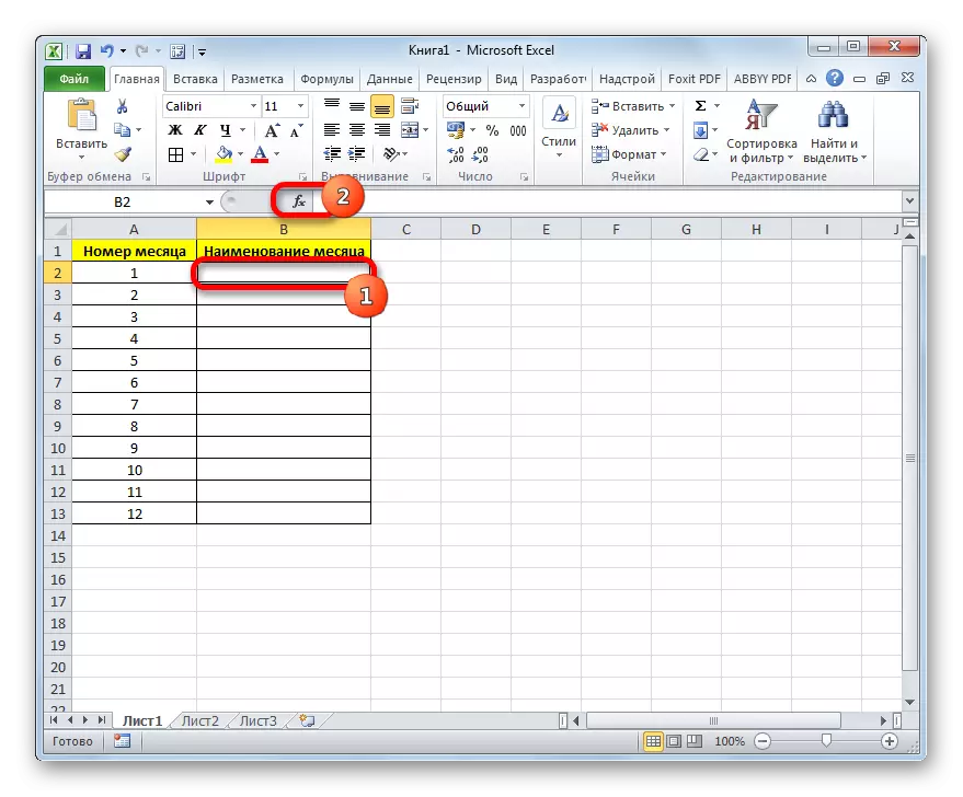
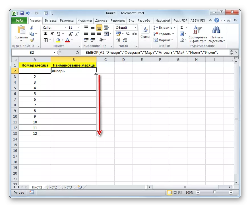
Let's see how this feature is valid on the simplest example. We have a table with numbering from 1 to 12. It is necessary according to these sequence numbers using the Select function to specify the name of the corresponding month in the second column of the table.

1. We highlight the first empty cell of the Column "Name of the Month". Click on the "Insert function" icon near the formula string.



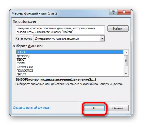
2. Running the wizard of functions. Go to the category "Links and arrays". Choose from the list the name "Select" and click on the "OK" button.



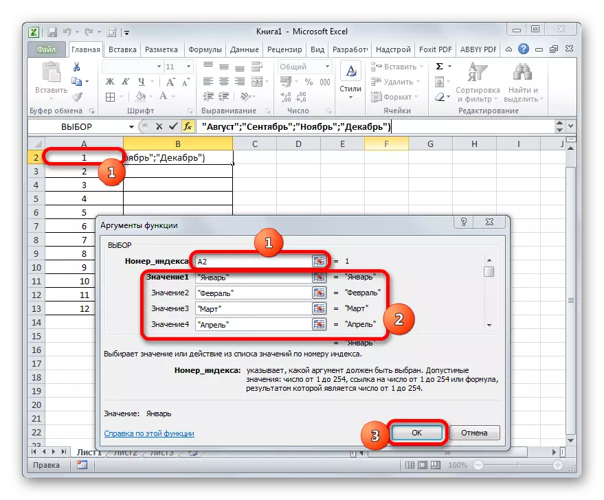
3. The Operator Arguments window is running. In the Index Number field, you should specify the address of the first cell number of the number of numbering. This procedure can be performed by manually driven by the coordinates. But we will do more conveniently. Install the cursor in the field and click the left mouse button along the corresponding cell on the sheet. As you can see, the coordinates are automatically displayed in the argument window field.

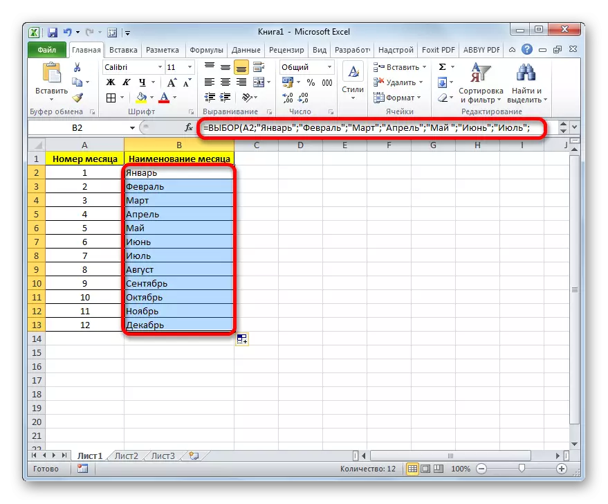
   After that, we have to manually drive the name of the months in the group of fields. Moreover, each field must correspond to a separate month, that is, in the "Value1" field, "January" is recorded in the field "D." - "February", etc.

   After executing the specified task, click on the "OK" button at the bottom of the window.



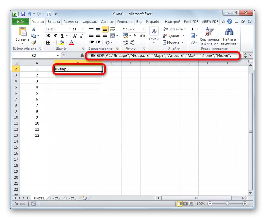
4. As you can see, immediately in the cell that we noted in the first action, the result was displayed, namely the name "January", corresponding to the first number of the month in the year.



5. Now, in order not to enter the formula for all other cells of the "Name of the Month" column, we will have to copy it. To do this, we install the cursor to the lower lower corner of the cell containing the formula. The filling marker appears. Click the left mouse button and pull the fill marker down to the end of the column.



6. As you can see, the formula was copied to the range we need. In this case, all the names of the months that were displayed in the cells correspond to their sequence number from the column on the left.

Lesson: Master of Functions in Excel

Example 2: Arbitrary elements arrangement

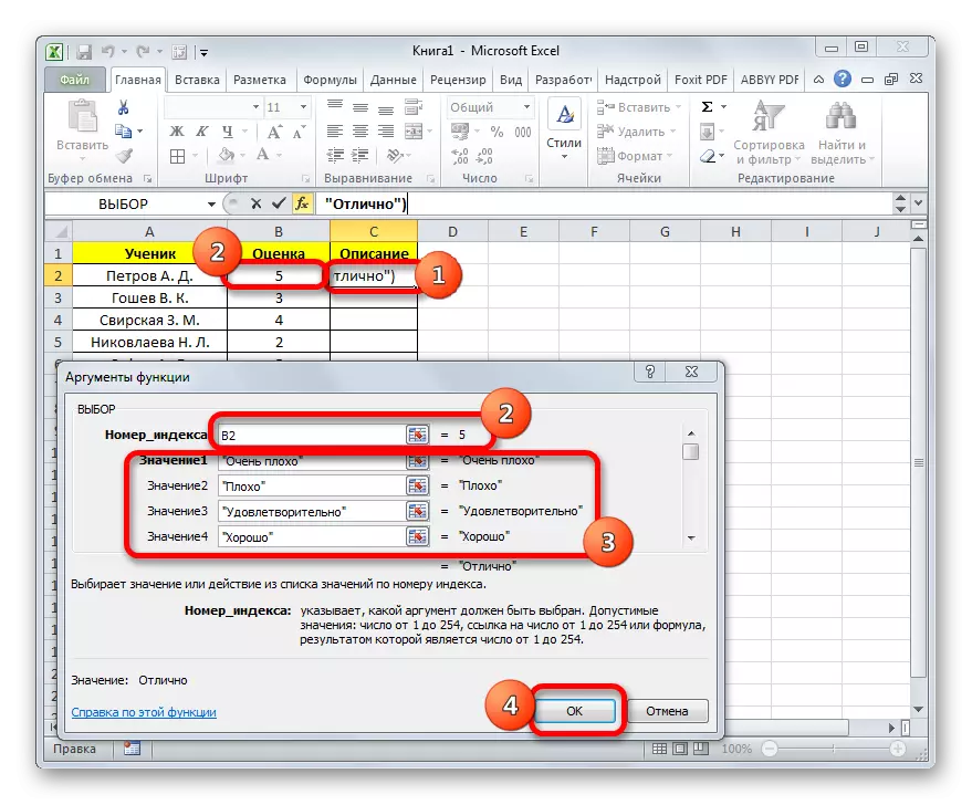
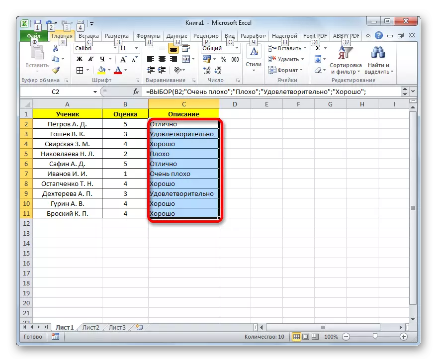
In the previous case, we applied the formula to choose when all values ​​of the index numbers were arranged in order. But how does this operator work in the case if the specified values ​​are mixed and repeated? Let's look at this on the example of the table with the performance of schoolchildren. In the first column of the table, the name of the student is indicated, in the second estimate (from 1 to 5 points), and in the third we will have a choice of the choice to give this estimate ("very bad", "bad", "satisfactory", "good" , "perfect").

1. We allocate the first cell in the "Description" column and move with the help of the method that the conversation has already been challenged is above, the choice of the selection window of the operator arguments.

   In the "Index number" field, specify a link to the first cell of the "Evaluation" column, which contains a score.

   Group of fields "Meaning" Fill as follows:

   • "Value1" - "very bad";
   • "Meaning2" - "bad";
   • "Meaning3" - "satisfactory";
   • "Value4" - "good";
   • "Value5" - "excellent."

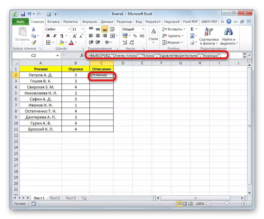
   After the introduction of the above data is manufactured, click on the "OK" button.



2. The score value for the first element is displayed in the cell.



3. In order to produce a similar procedure for the remaining column elements, copy the data in its cells using the filling marker, as was done in the method 1. As we see, and this time the function worked correctly and output all the results in accordance with the specified algorithm.

Example 3: Use in combination with other operators

But much more productive the selection operator can be used in combination with other functions. Let's see how this is done on the example of the application of the operators and sums.

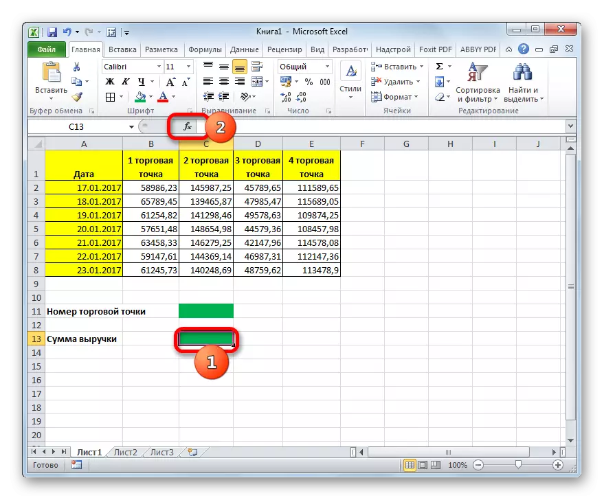
There is a product sales table. It is divided into four columns, each of which corresponds to a specific trading point. Revenue is indicated separately for a specific date line. Our task is to make it so that after entering the number of the outlet in a certain cell of the sheet, the amount of revenue for all the days of the specified store was displayed. For this we will use a combination of state operators and choosing.

1. Select the cell in which the result will be output. After that, click on the already familiar to us the "Insert function" icon.



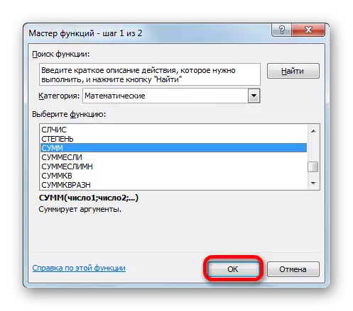
2. The functions wizard window is activated. This time we move to the category "Mathematical". We find and allocate the name "sums". After that, click on the "OK" button.



3. The window of the arguments of the function arguments are launched. This operator is used to count the amount of numbers in the sheet cells. Its syntax is quite simple and understandable:

   = Sums (number1; number2; ...)

   That is, the arguments of this operator are usually either numbers or, even more often, references to cells where contains the numbers that need to be summed up. But in our case, in the form of a single argument, not the number and not the link, but the content of the function function.

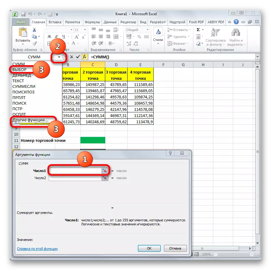
   Install the cursor in the "Number1" field. Then click on the icon, which is depicted in the form of an inverted triangle. This icon is in the same horizontal row where the "Insert function" button and the formula string are located, but to the left of them. A list of newly used features is available. Since the formula selection was recently used by us in the previous method, it is available on this list. Therefore, it is enough to click on this item to go to the argument window. But it is more likely that you will not be in the list of this name. In this case, you need to click on the "Other functions ..." position.



4. The wizard of the functions is launched, in which in the "Links and Arrays" section we must find the name "Choice" and allocate it. Click on the "OK" button.



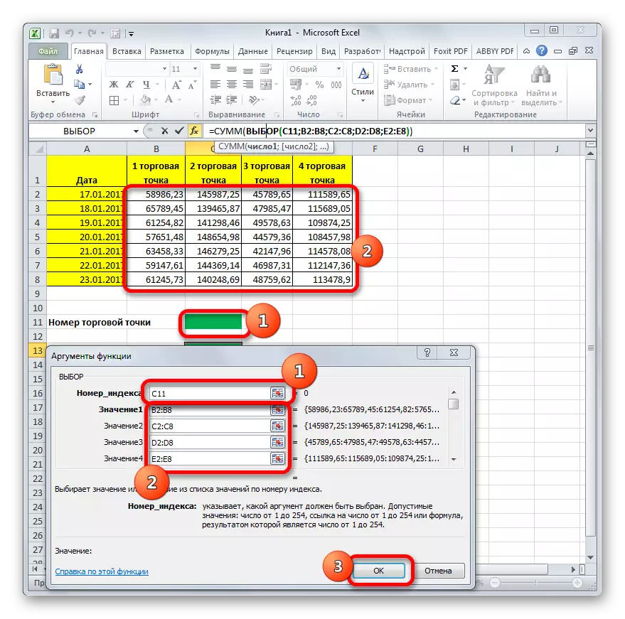
5. The operator arguments selection window is activated. In the "Index Number" field, specify the link to the cell of the sheet, in which we enter the number of the trading point for the subsequent display of the total amount of revenue.

   In the "Value1" field, you need to enter the coordinates of the "1 shopping point" column. Make it is quite simple. Install the cursor in the specified field. Then, holding the left mouse button, we allocate the entire range of the cells of the column of the "1 shopping point". The address will immediately appear in the argument window.

   Similarly, in the "Value2" field, add the coordinates of the column "2 shopping point", in the "value3" field - "3 trading point", and in the "Value" field - "4 trading point".

   After performing these actions, press the "OK" button.



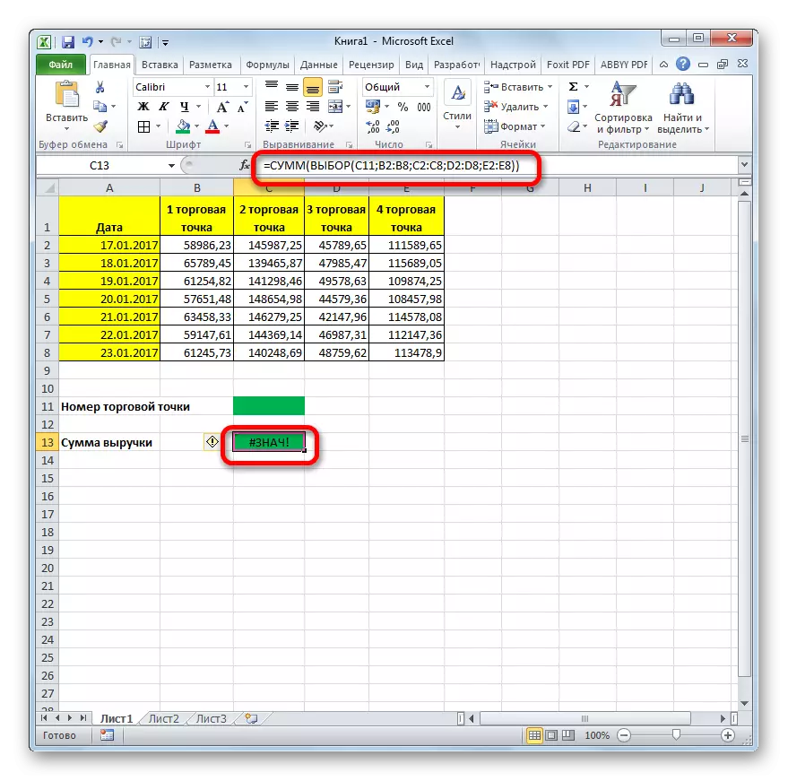
6. But, as we see, the formula displays the erroneous meaning. This is due to the fact that we have not yet entered the number of the trading point to the appropriate cell.



7. We enter the number of the trading point in the cell intended for these purposes. The amount of revenue by the appropriate column is immediately displayed in the sheet element in which the formula is installed.

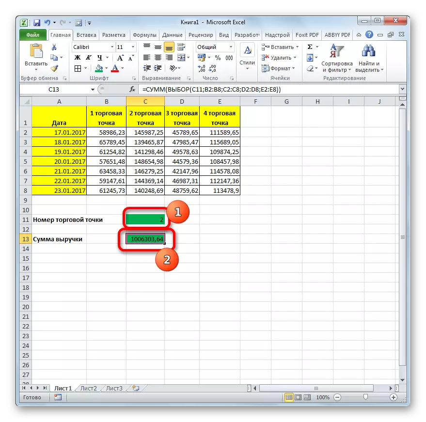
It is important to consider that you can enter only numbers from 1 to 4, which will correspond to the number of the outlet. If you enter any other number, then the formula will return an error again.

Lesson: How to calculate the amount in Excel

As you can see, the choice function with its proper application may become a very good helper to perform the tasks. When using it in combination with other operators, the ability to significantly increase.