ABC Analysis in Excel

One of the key methods of management and logistics is ABC analysis. With it, you can classify the resources of the enterprise, goods, customers, etc. According to the degree of importance. At the same time, by the level of importance, each of the above unit is assigned one of three categories: A, B or C. Excel program has in its baggage tools that make it easier to carry out this kind of analysis. Let's figure out how to use them, and what is the ABC analysis.

Using ABC analysis

ABC analysis is a kind of enhanced and adapted to modern conditions for the Pareto principle. According to the method of its conduct, all elements of the analysis are divided into three categories according to the degree of importance:

• Category A - elements having a combination of more than 80% of specific gravity;
• Category B - elements whose combination ranges from 5% to 15% of specific gravity;
• Category C - the remaining elements, the total aggregate of which is 5% and less specific gravity.

Separate companies use more advanced techniques and divide items not to 3, but by 4 or 5 groups, but we will rely on the classic ABC analysis scheme.

Method 1: Analysis with sorting

Excel ABC analysis is performed using sorting. All items are sorted from greasy to less. Then the accumulative share of each element is calculated, on the basis of which it is assigned a certain category. Let's find out how the specified methodology is used in practice.

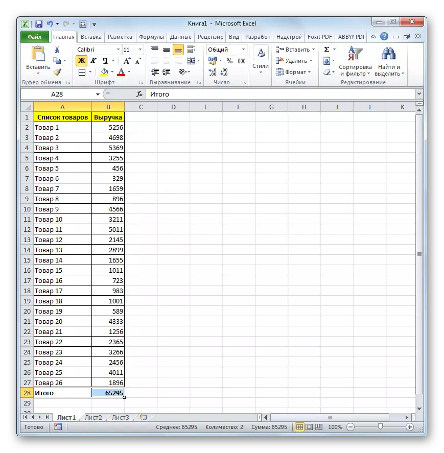
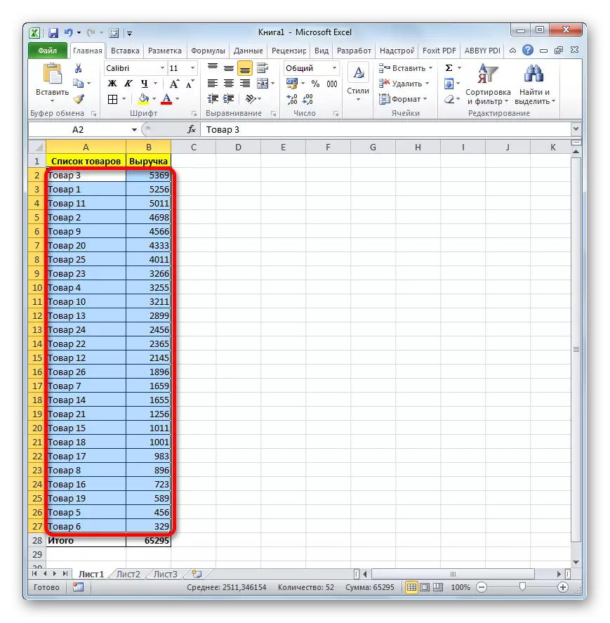
We have a table with a list of products that the company sells, and the corresponding number of revenues from their sale for a certain period of time. At the bottom of the table, the outcome of the revenue in general on all the names of the goods. There is a task using ABC analysis, break these goods into groups by their importance for the enterprise.

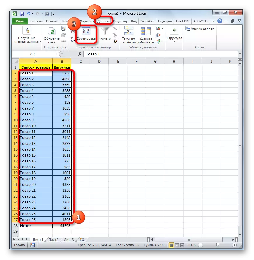
1. We highlight a table with the cursor by closing the left mouse button, excluding the cap and the final string. Go to the "Data" tab. We click on the "Sort" button, located in the "Sort and Filter" toolbar on the tape.

   

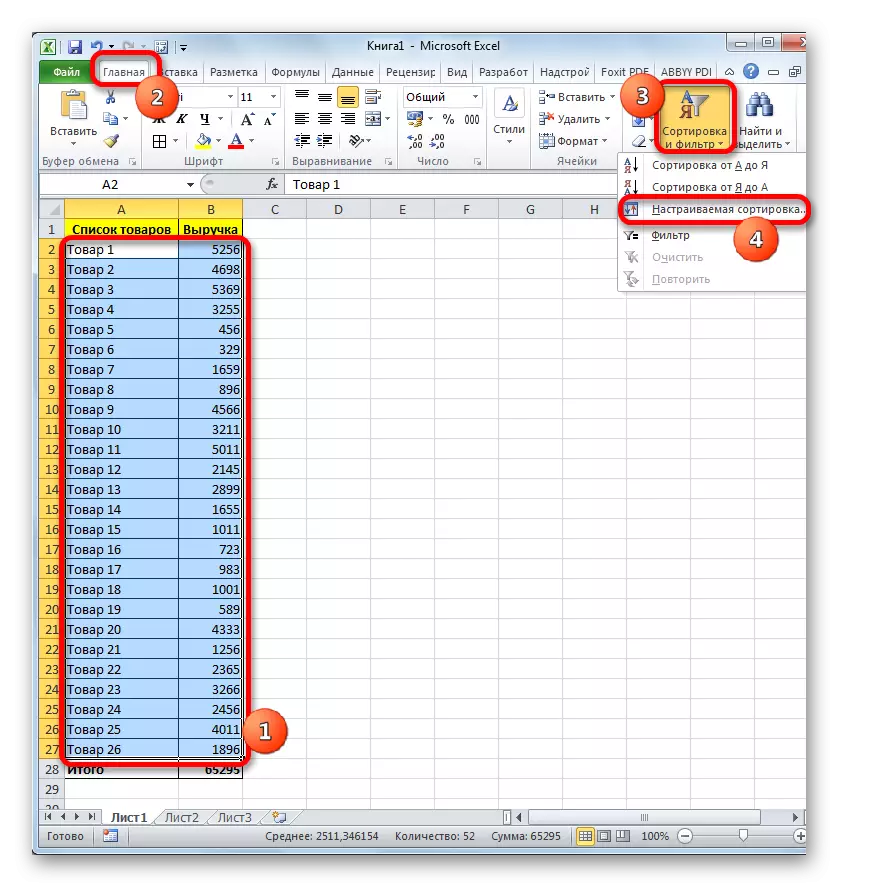
   You can also do differently. We allocate the above table range, then move to the "Home" tab and click on the "Sort and Filter" button located in the Editing toolbox on the tape. The list is activated in which the position "Customizable Sorting" is activated.



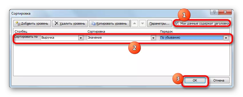
2. When applying any of the above actions, the Sorting Settings window launches. We look so that the "My Data contains the headers" parameter was set to a check mark. In the case of its absence, install.

   In the "Column" field, specify the name of the column in which the revenue data is contained.

   In the "Sort" field, you need to specify, on which specific criteria will be sorted. Leave the preset settings - "Values".

   In the "order" field, exhibit the position "descending".

   After the product of the specified settings, click on the "OK" button at the bottom of the window.



3. After performing the specified action, all items were sorted by revenue from more to a smaller.



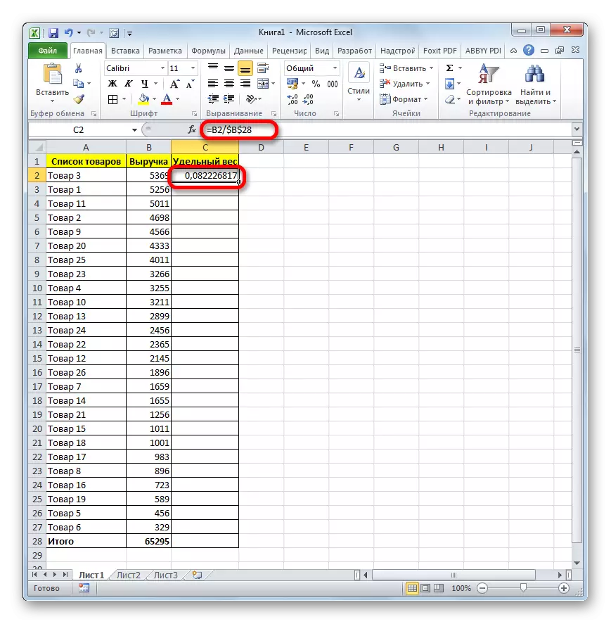
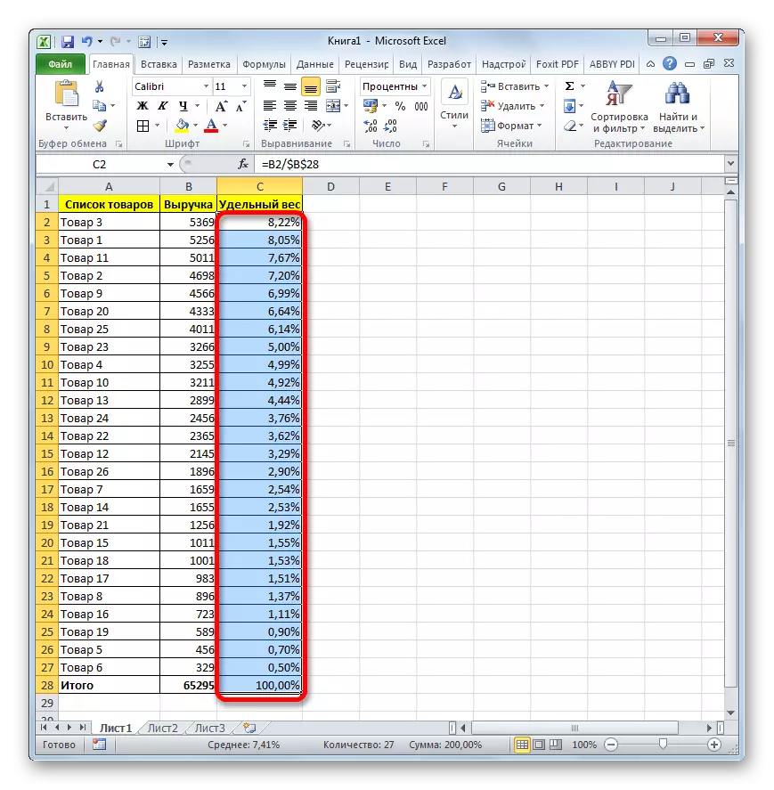
4. Now we should calculate the proportion of each of the elements for a general result. Create an additional column for these purposes, which we call "share weight". In the first cell of this column, we put the sign "=", after which you specify a link to the cell in which the amount of revenue from the implementation of the relevant product is. Next, set the sign of the division ("/"). After that, we indicate the coordinates of the cell, which contains the total amount of the sale of goods throughout the enterprise.

   Given the fact that the specified formula we will copy to other cells of the "share" column by the filling marker, the address of the link to the element containing the final amount of revenue to the enterprise, we need to fix. To do this, make a link absolute. Select the coordinates of the specified cell in the formula and press the F4 key. Before the coordinates, as we see, a dollar sign appeared, which indicates that the link has become absolute. It should be noted that the reference to the amount of revenue of the first in the list of goods (product 3) should remain relative.

   Then, to make calculations, press the ENTER button.



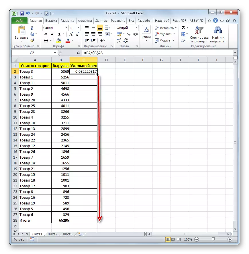
5. As we see, the proportion of revenue from the first product specified in the list appeared in the target cell. To copy the formula in the range below, we put the cursor to the lower right corner of the cell. Its transformation in the filling marker, having a look of a small cross. We click the left mouse button and drag the fill marker down to the end of the column.



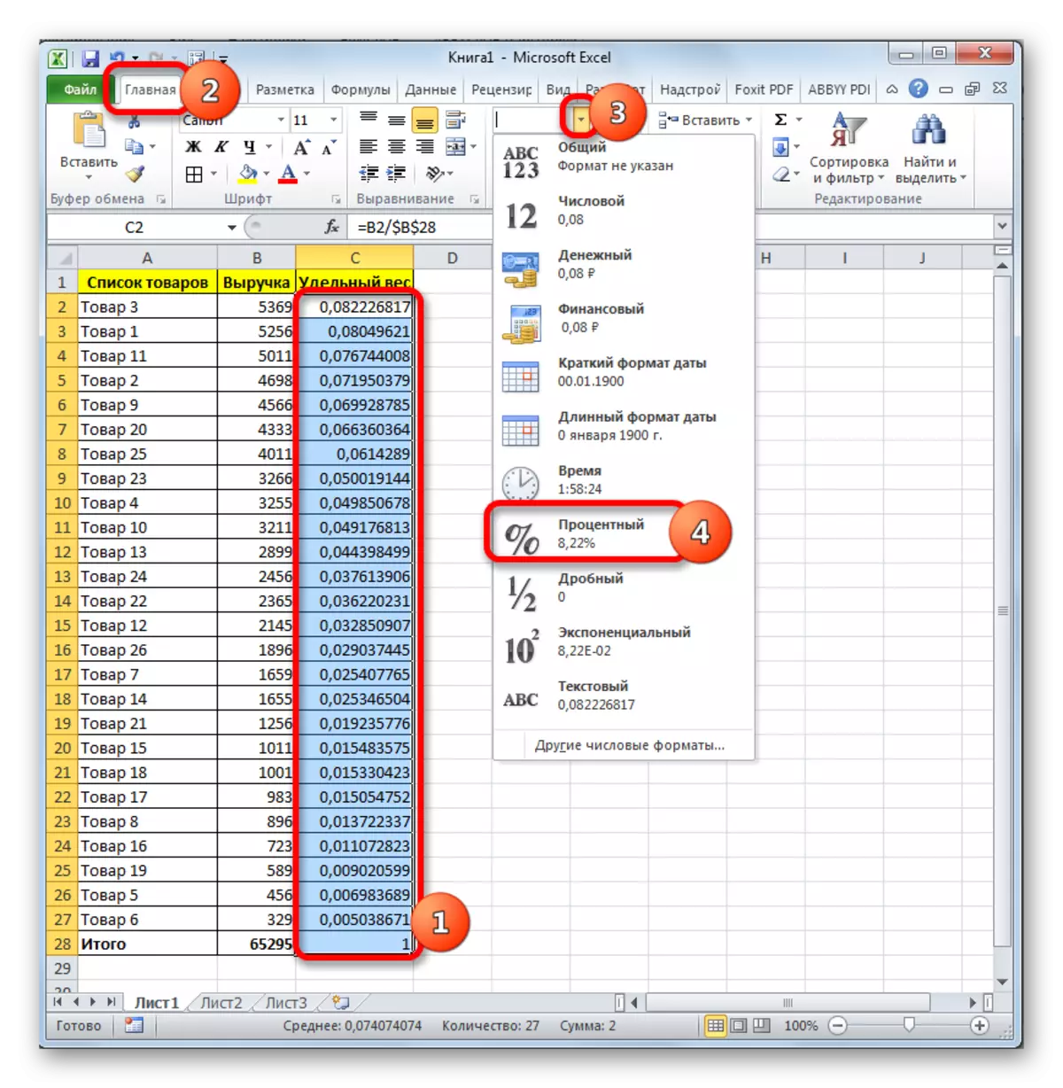
6. As you can see, the entire column is filled with data characterizing the proportion of revenue from the implementation of each product. But the value of the specific gravity is displayed in the numerical format, and we need to transform it into percentage. To do this, highlight the contents of the column "specific weight". Then we move to the "Home" tab. On the tape in the group settings group there is a field displaying data format. By default, if you did not produce additional manipulations, the "General" format must be installed there. Click on the icon in the form of a triangle located on the right of this field. In the list of formats, select the "percentage" position.



7. As we see, all the column values ​​were transformed into percentage values. As it should be, 100% indicated in the string of "Total". The share of goods is expected in the column from a larger to a smaller.



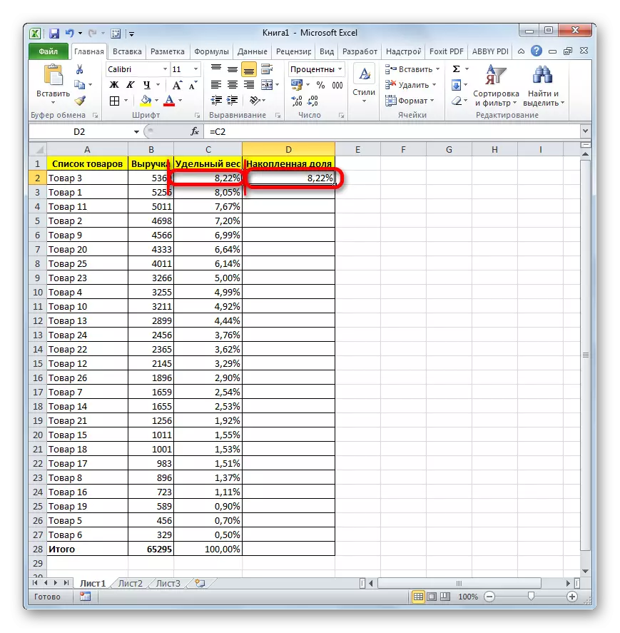
8. Now we should create a column in which the accumulated share with a growing outcome would be displayed. That is, in each line to the individual specific weight of a specific product will be added the proportion of all those products that are located in the list above. For the first goods in the list (Product 3), individual proportion and accumulated share will be equal, but all subsequent to the individual indicator will need to add the accumulated share of the previous element of the list.

   So, in the first line we are transferred to the column "accumulated share" the indicator of the column "Specific".



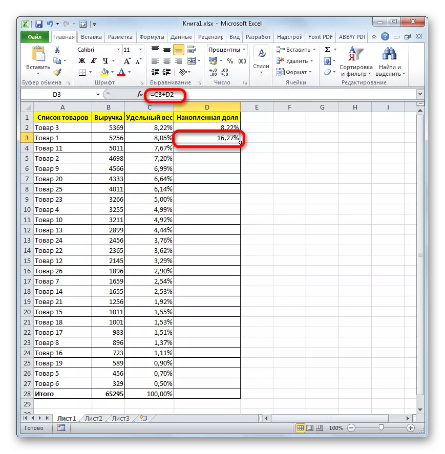
9. Next, set the cursor to the second cell of the "accumulated share" column. Here we have to apply the formula. We put the sign "equal" and fold the contents of the cell "The proportion" of the same line and the contents of the cell "accumulated share" from the string above. All references are reserved relative, that is, we do not produce any manipulations with them. After that, perform a click on the ENTER button to display the final result.



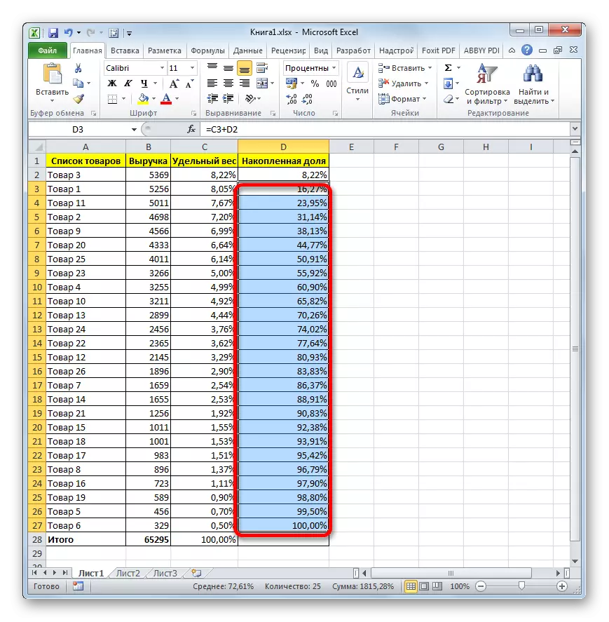
10. Now you need to copy this formula in the cells of this column, which are placed below. To do this, we use the filling marker to which we have already resorted when copying the formula in the share column. At the same time, the string "Total" is not necessary, since the accumulated result is 100% will be displayed on the last product from the list. As you can see, all the elements of our column after that were filled.



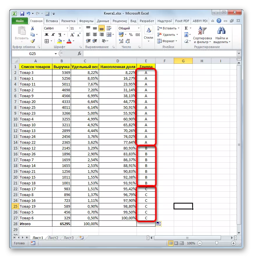
11. After that, create a column "Group". We will need to group goods by category A, B and C according to the specified accumulated share. As we remember, all elements are distributed by groups according to the following scheme:
    • A - up to 80%;
    • B - the following 15%;
    • C - the remaining 5%.

    Thus, all goods that accumulated share of the specific weight of which is within the border of up to 80%, we assign category A. The goods with the accumulated specific weight from 80% to 95% are assigned to the category B. The remaining group of goods with the value of more than 95% of the accumulated specific gravity we assign a category C.



12. For clarity, you can fill the specified groups with different colors. But it is at will.

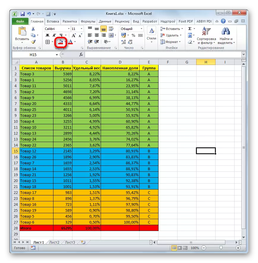
Thus, we broke the elements on the level of importance, using ABC analysis. When using some other techniques, as mentioned above, it is used to break into a larger number of groups, but the principle of breaking in this case remains almost unchanged.

Lesson: Sorting and filtering in Excel

Method 2: Using a complex formula

Of course, the use of sorting is the most common way to conduct ABC analysis in Excele. But in some cases it is necessary to carry out this analysis without rearranging lines in places in the source table. In this case, a complex formula will come to the rescue. For example, we will use the same source table as in the first case.

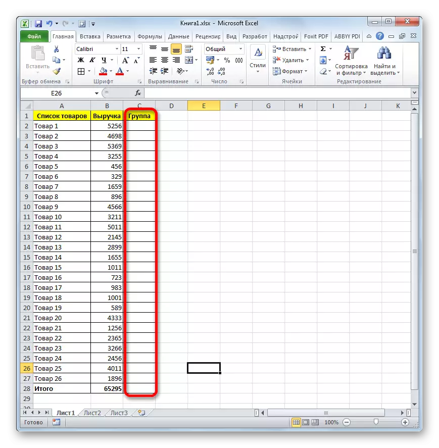
1. We add to the source table containing the name of the goods and the revenue from the sale of each of them, the Column "Group". As you can see, in this case, we may not add columns with the calculation of individual and accumulative fractions.



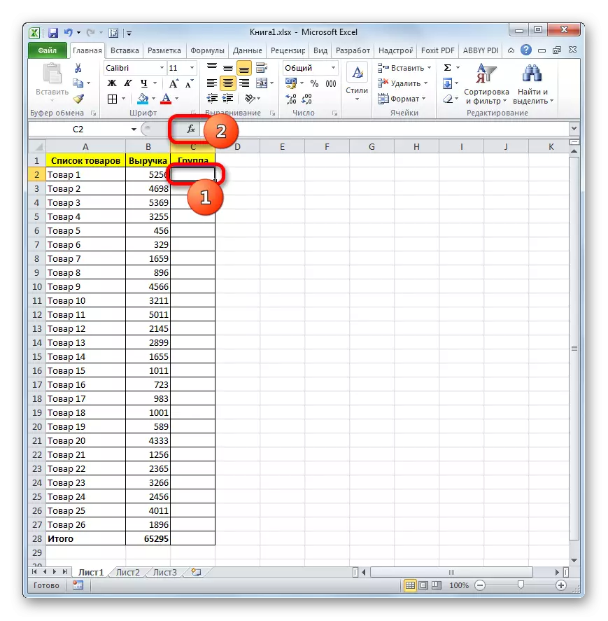
2. We produce the first cell allocation in the group column, after which you perform a click on the "Insert function" button located near the formula row.



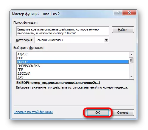
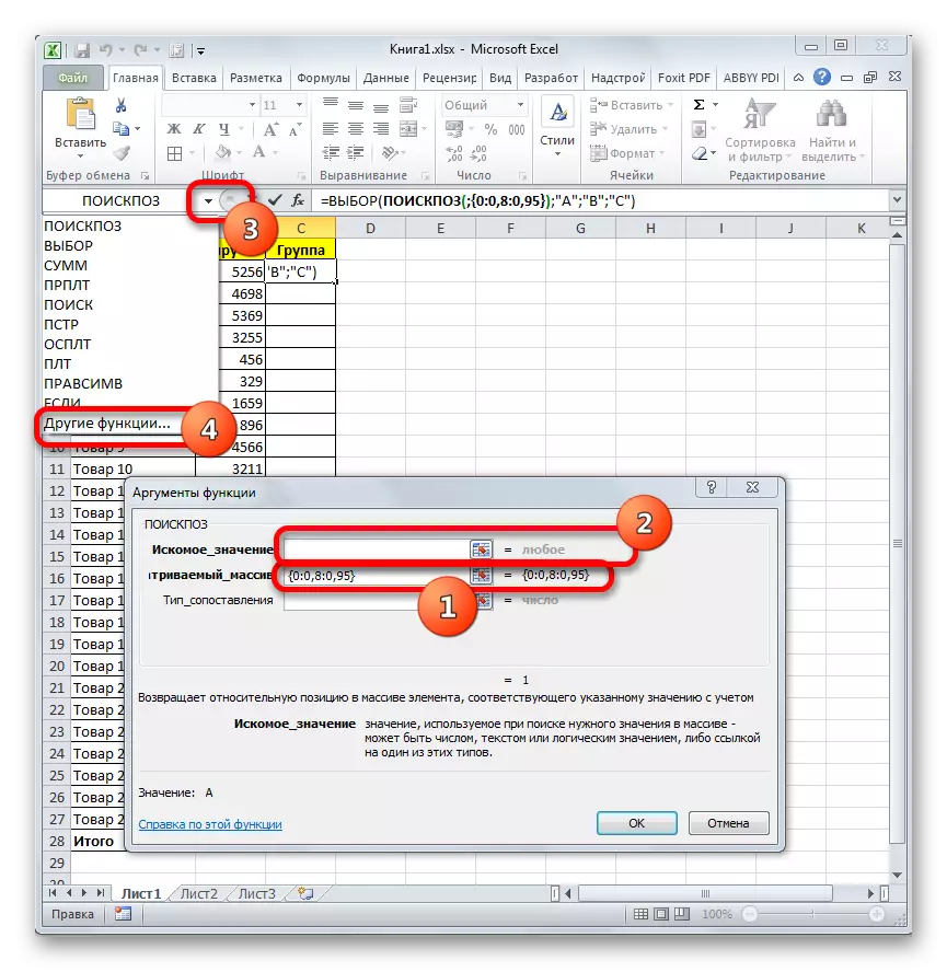
3. Masters activation of functions. We move to the category "Links and arrays". Select the "Choice" function. We make a click on the "OK" button.



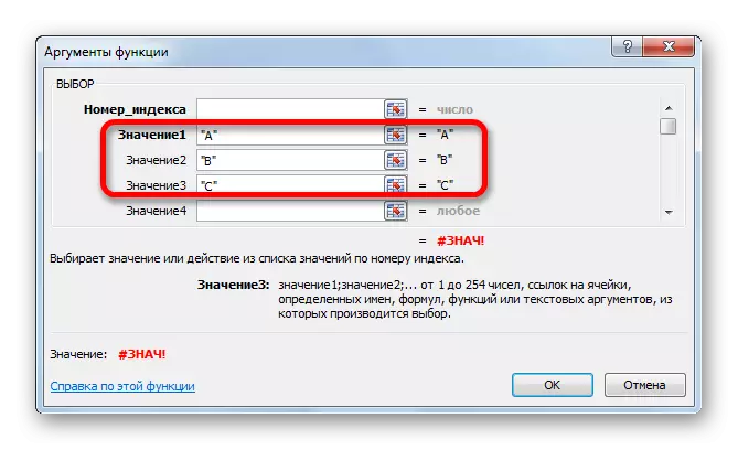
4. The game argument window is activated. The syntax is presented as follows:

   = Selection (number_intex; value1; value2; ...)

   The task of this feature is the withdrawal of one of the specified values, depending on the index number. The number of values ​​can reach 254, but we will need only three names that correspond to ABC-analysis categories: A, B, C. We can immediately enter the "A" symbol in the "B" field in the "B" field, Field "Value3" - "C".



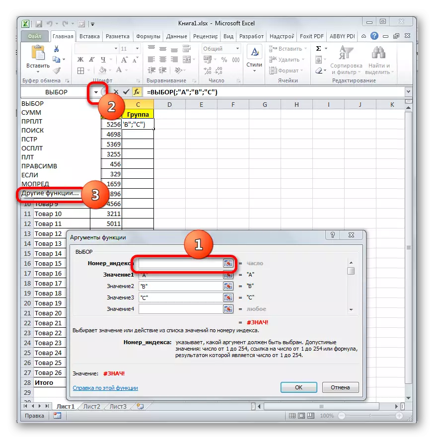
5. But the argument "index number" have thoroughly tinker, build in it a few additional operators. Set the cursor to the "index number". Next, click on the icon form of a triangle to the left of the button "Insert Function". It opens a list of recently used by operators. We need a function MATCH. Since the list it is not, then click on the label "Other features ...".



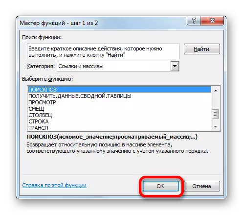
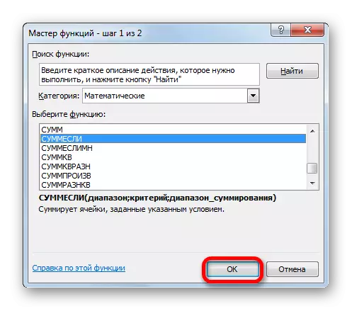
6. Again produced a startup wizard window functions. Again, go to the category "References and Arrays." We find there the position of "MATCH", select it and do click on «OK» button.



7. A window opens MATCH operator arguments. its syntax is as follows:

   MATCH = (lookup_value lookup_array; match_type)

   Purpose of this function - the definition of the position number of the element. That is just what we need for the field "index number" function selection.

   In the "Browse an array of" immediately, you can specify the following expression:

   {0: 0.8: 0.95}

   It should be just in braces, as an array formula. Not difficult to understand that these numbers are (0; 0.8; 0.95) indicate the borders between the groups of the accumulated fraction.

   The "Match type" is not compulsory and in this case we will not fill.

   In the "correct value" set cursor. Then again through the above icon in the shape of a triangle are moving in the Function Wizard.



8. At this time the wizard function is moving in the category "Math". Choosing the name "SUMIF" and click on the button «OK».



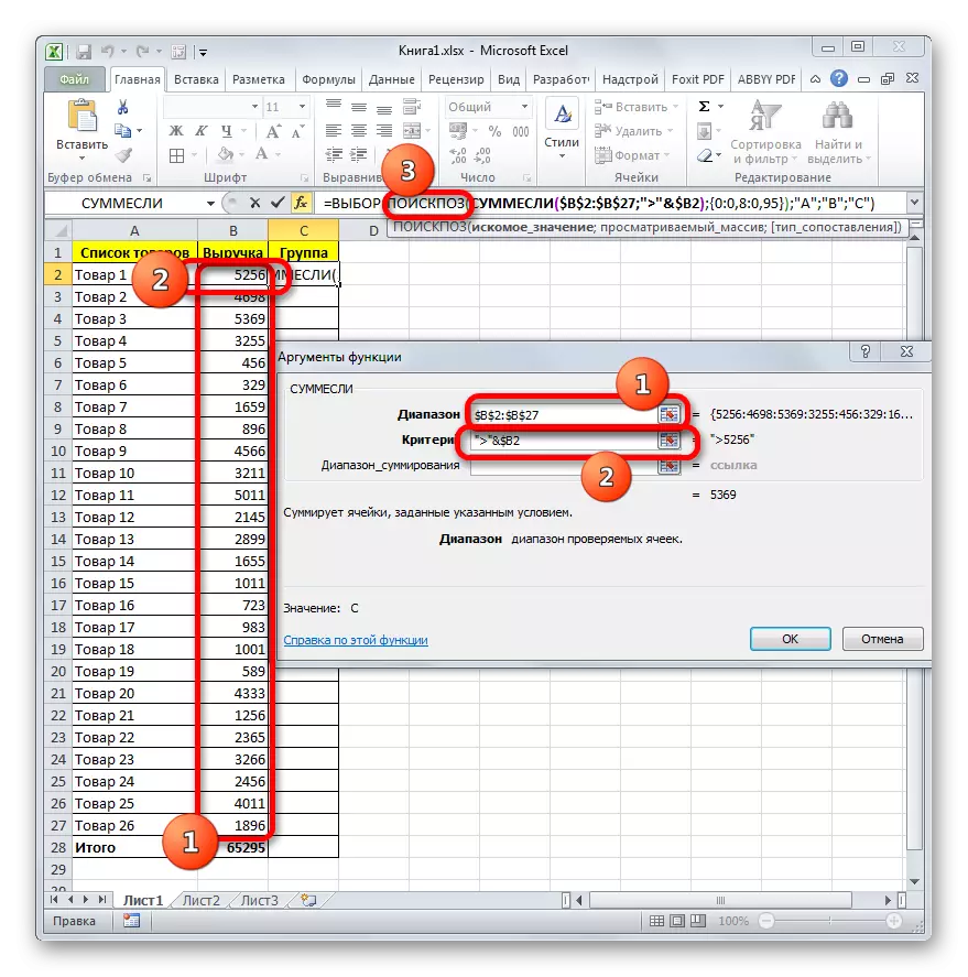
9. The function arguments window will be launched. The above statement sums up the cells that meet a certain condition. Its syntax is as follows:

   = SUMIF (range criterion; sum_range)

   In the "Range", enter the address of the column "Revenue". For this purpose, set the cursor in the field, and then, making the clip with the left mouse button, select all the relevant cells of the column, excluding the value of "Total". As you can see, the address immediately displayed in the field. In addition, we need to make this an absolute link. To do this, we make its selection and click on the F4. Address allocated $ signs.

   In the "criterion", we need to define the condition. We enter the following expression:

   ">"&

   Then, immediately after the address of the first skid column cell "Revenue". We are making the horizontal coordinates in the absolute address by writing a letter to the dollar sign from the keyboard. Coordinates vertically relative reserve, that is, should not be before the number is no sign.

   After that, do not click on the button «OK», and click on the name MATCH function in the formula bar.



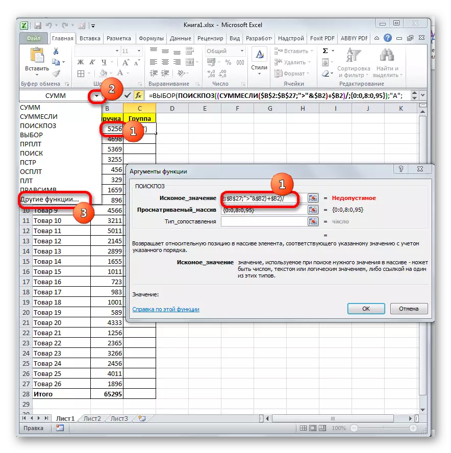
10. Then we return to the window of arguments MATCH. As you can see, in the "correct value" there is evidence given SUMIF operator. But that is not all. Move into this field and by reportedly adding a "+" without the quotes. Then make the cell address of the first column "Revenue". Again, we do the coordinates of the horizontal links of the absolute and relative vertical reserve.

    Next, we take all the content of the "required value" in brackets, after which the set division sign ( "/"). Then again through the triangle icon to turn the function selection window.



11. As with the last time the right operator looking in the Function Wizard in the category "Math". At this time, the desired function is called the "sum". Select it and click on the button «OK».



12. A window opens SUM operator arguments. Its main purpose - is the summation of data in cells. The syntax is quite simple:

    = SUM (number1; number2; ...)

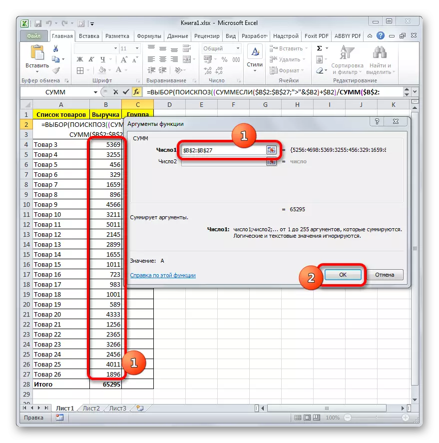
    "Number 1" field only need for our purposes. Was added thereto column coordinate range "Revenue", eliminating a cell that contains the results. Such an operation we have carried out in the field "Range" SUMIF function. As at that time, the coordinates of the range do absolutely by highlighting them and pressing the F4 key.

    After that click on the button «OK» at the bottom of the window.



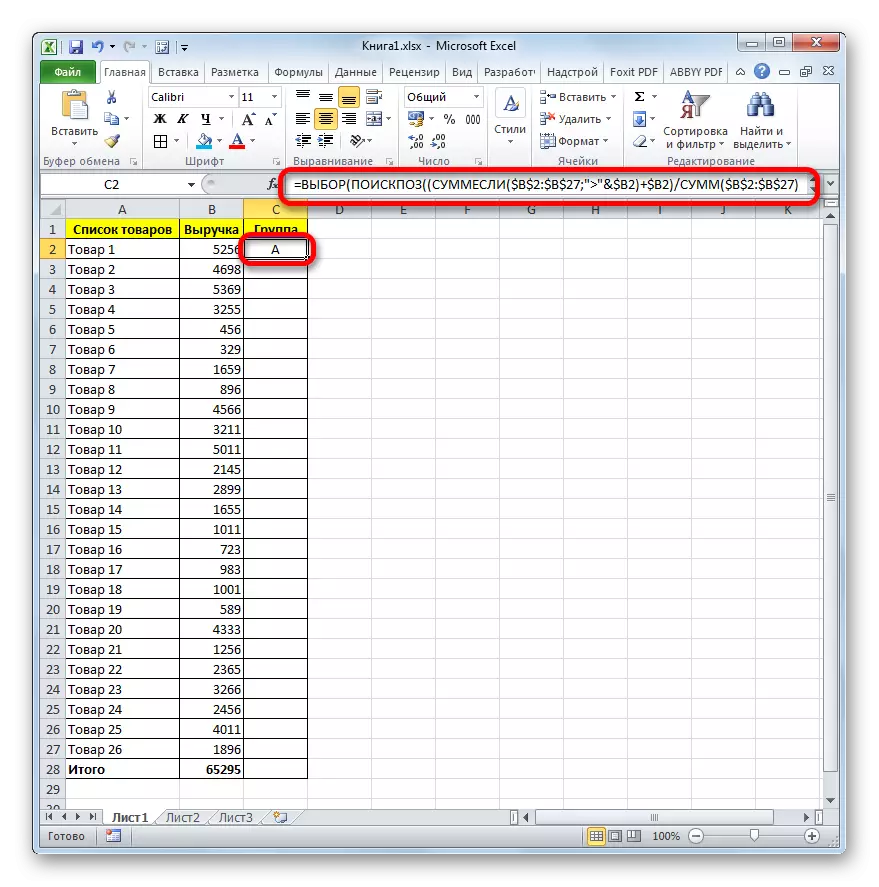
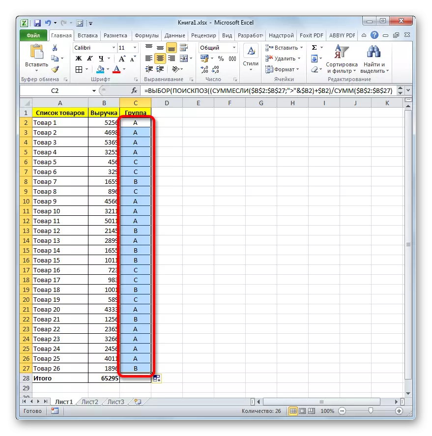
13. As you can see, the complex of the above functions has made the calculation and outputs the result to the first cell in the column "Group". «A» group was assigned to the first product. Complete formula, we applied for this calculation is as follows:

    = CHOOSE (MATCH ((SUMIF ($ B $ 2: $ B $ 27; ">" & $ B2) + $ B2) / SUM ($ B $ 2: $ B $ 27); {0: 0.8: 0.95} ); "A"; "B"; "C")

    But, of course, in each particular case, the coordinates in the formula will vary. Therefore, it can not be considered universal. But, using the guide, which has been given above, you can insert the coordinates of any of the table and successfully applied this method in any situation.



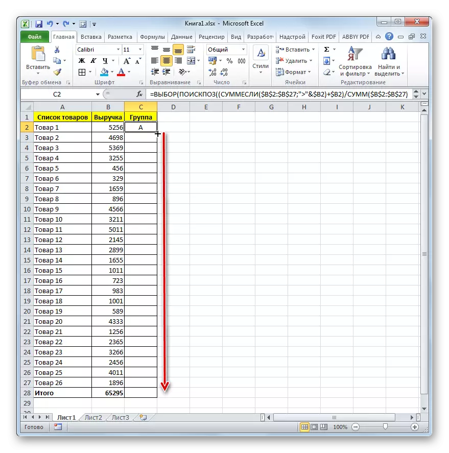
14. However, that's not all. We made a calculation for the first row of the table only. In order to fully populate the column "Group", you need to copy this formula into the range below (excluding the cell line "Total") using the fill handle, as we have done many times. After the data has been entered, ABC-analysis can be considered fulfilled.

As we see, the results obtained using the option using a complex formula are not different from those results that we were performed by sorting. All the goods are assigned the same categories, only at the same time the rows did not change their initial position.

Lesson: Master of Functions in Excel

The Excel program is able to significantly alleviate ABC analysis for the user. This is achieved by using such a tool as sorting. After that, the individual specific gravity, accumulated share and, actually, partitioning into groups is calculated. In cases where the change in the initial position of the rows in the table is not allowed, you can apply the method using a complex formula.