Correlation analysis in Excel: 2 work options

Correlation analysis is a popular method of statistical research, which is used to identify the degree of dependence of one indicator from the other. Microsoft Excel has a special tool designed to perform this type of analysis. Let's find out how to use this function.

The essence of correlation analysis

The purpose of the correlation analysis is reduced to identifying the dependence between different factors. That is, it is determined whether the decrease is influenced or an increase in one indicator on the change in the other.

If the dependence is established, the correlation coefficient is determined. Unlike regression analysis, this is the only indicator that calculates this method of statistical research. The correlation coefficient varies in the range from +1 to -1. If there is a positive correlation, an increase in one indicator contributes to an increase in the second. With a negative correlation, an increase in one indicator entails a decrease in the other. The greater the correlation coefficient module, the more visible change in one indicator is reflected on the change in the second. With a coefficient equal to 0, the dependence between them is completely absent.

Calculation of the correlation coefficient

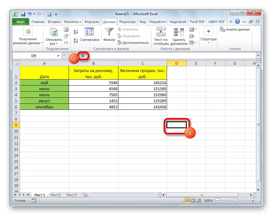
Now let's try to calculate the correlation coefficient on a specific example. We have a table in which it is monthly painted in separate speakers for advertising costs and sales. We have to find out the degree of dependence of the number of sales from the amount of funds, which was spent on advertising.

Method 1: Determining the correlation through the Master of Functions

One way to which the correlation analysis can be carried out is to use the correlation function. The function itself has a general view of the corneal (array1; array2).

1. Select the cell in which the result of the calculation should be output. Click on the "Insert function" button, which is placed on the left of the formula string.



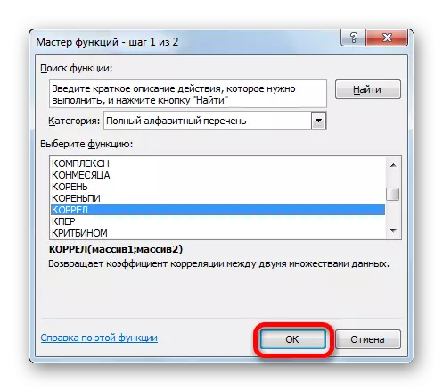
2. In the list, which is presented in the Wizard Wizard, we look for and allocate the function of the cornel. Click on the "OK" button.



3. The function arguments opens. In the "Massive1" field, we introduce the coordinates of the range of cells of one of the values, whose dependence should be determined. In our case, these will be values ​​in the "Sales" column. In order to add an array address in the field, simply allocate all cells with data in the above column.

   In the field "Massive2" you need to make coordinates of the second column. We have advertising costs. Just as in the previous case, we entered the data in the field.

   Click on the "OK" button.

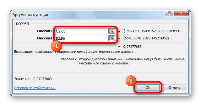
As we see, the correlation coefficient in the form of a number appears in the cell that we selected. In this case, it is equal to 0.97, which is a very high feature of the dependence of one value from the other.

Method 2: Calculating the correlation using a package of analysis

In addition, the correlation can be calculated using one of the tools, which is represented in the analysis package. But before we need this tool to activate.

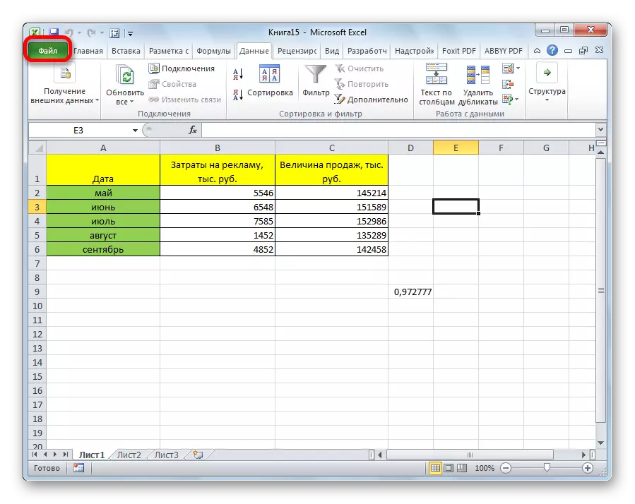
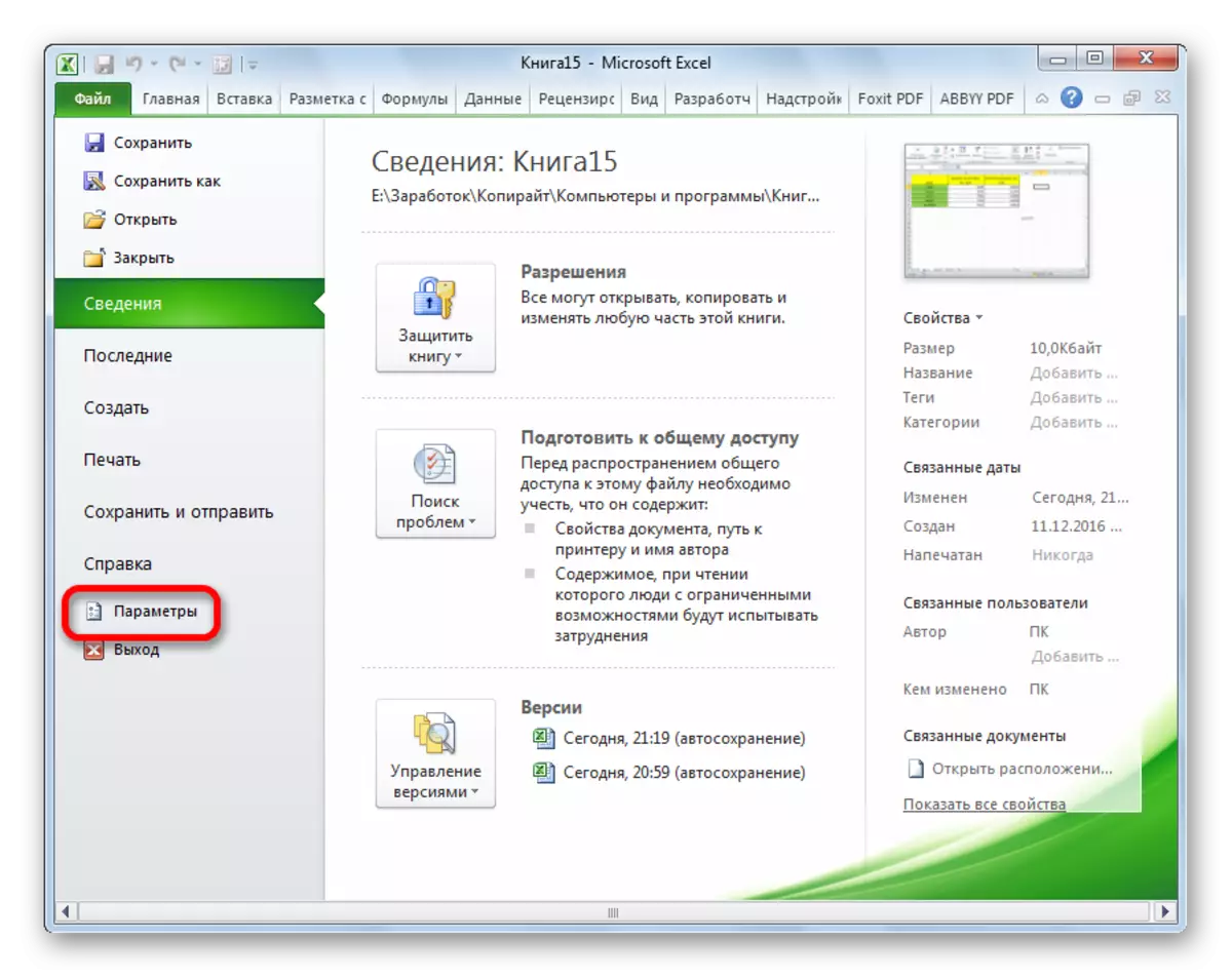
1. Go to the "File" tab.



2. In the window that opens, move to the "Parameters" section.



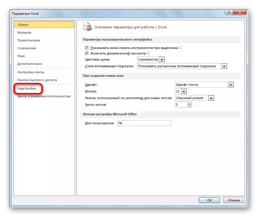
3. Next, go to the "Add-in".



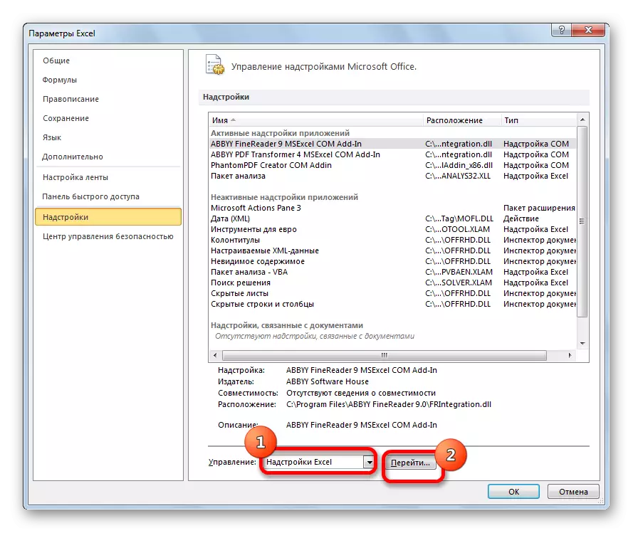
4. At the bottom of the next window in the "Management" section, we rearrange the switch to the "Excel add-in" position, if it is in another position. Click on the "OK" button.



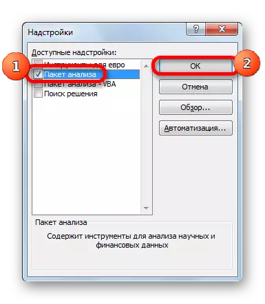
5. In the window of the add-ons, we install a tick near the "Analysis Package" item. Click on the "OK" button.



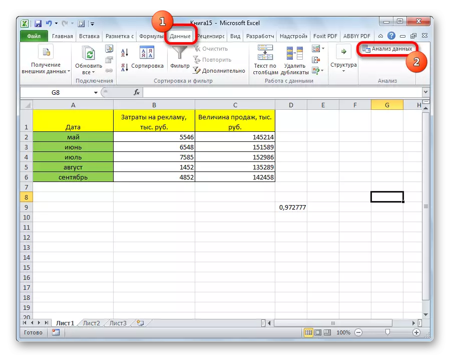
6. After that, the analysis package is activated. Go to the "Data" tab. As you can see, a new tool block appears on the ribbon - "Analysis". Click on the "Data Analysis" button, which is located in it.



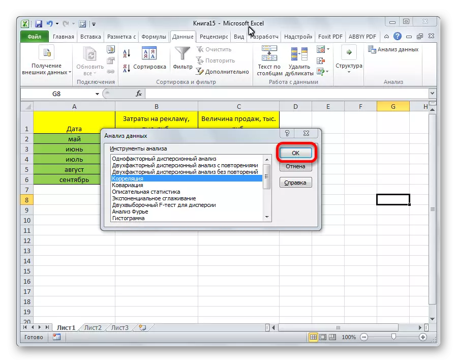
7. A list with various data analysis options. Select the point "Correlation". Click on the "OK" button.



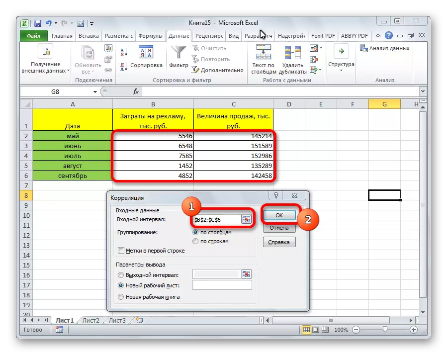
8. A window opens with correlation analysis parameters. In contrast to the previous method, in the field "Input interval" we introduce the interval of not each column separately, but all columns that are involved in the analysis. In our case, these are data in the columns "advertising costs" and the "sales value".

   The "Grinding" parameter is left unchanged - "on columns", since we have a data group broken into two columns. If they were broken line, then therefore should be rearranged the switch to the position "on the rows".

   In the default output parameters, the "New Work List" item is set, that is, the data will be displayed on another sheet. You can change the location by rearring the switch. It can be a current sheet (then you will need to specify the coordinates of information output cells) or a new working book (file).

   When all settings are set, click on the "OK" button.

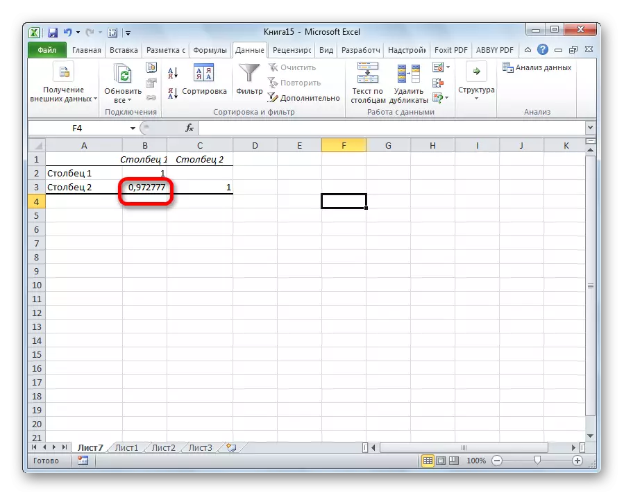
Since the analysis of the results of the analysis was left by default, we move to a new sheet. As you can see, the correlation coefficient is indicated. Naturally, he is the same as when using the first method - 0.97. This is explained by the fact that both options perform the same calculations, simply produce them in different ways.

As you can see, the Excel app offers two ways of correlation analysis at once. The result of the calculations, if you do everything correctly, will be completely identical. But, each user can choose a more convenient embodiment for it.