Criteria in Excel

The Microsoft Excel program is not just a tabular editor, but also a powerful application for various calculations. Not least this possibility has appeared thanks to the built-in features. With the help of some functions (operators), you can even set the calculation conditions that are called criteria. Let's find out in more detail how you can use them when working in Excele.

Application of criteria

Criteria are the conditions under which the program performs certain actions. They apply in a number of built-in functions. In their name, the expression "if" is most often present. To this group of operators, first of all, it is necessary to attribute the countdown, countableness, silemli, Sumymbremlin. In addition to embedded operators, the criteria in Excel are also used in conditional formatting. Consider their application when working with various tools of this tabular processor in more detail.

Countess

The main task of the operator's account belonging to the statistical group is counting employed by various cell values ​​that satisfy a specific given condition. Its syntax is as follows:

= Schedules (Range; Criterion)

As we see, this operator has two arguments. The "range" represents the address of an array of elements on a sheet in which the calculation should be calculated.

"Criterion" is an argument that sets the condition that it should contain the cells of the specified area to be included in the counting. A numeric expression, text or link to a cell in which the criterion is contained can be used as a parameter. At the same time, the following signs can be used to specify the criterion: "" ("" More ")," = "(" equal ")," "(" not equal "). For example, if you specify the expression "

And now let's see the example, as this operator works in practice.

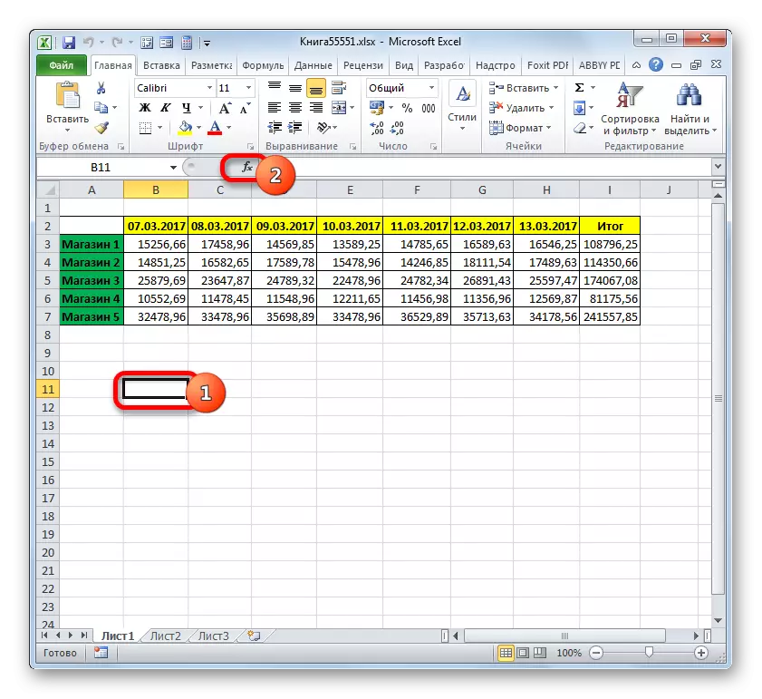
So, there is a table where revenue is prevented on five stores per week. We need to know the number of days for this period, in which in the store 2 income from sales exceeded 15,000 rubles.

1. Select the leaf element in which the operator will display the result of the calculation. After that, click on the "Insert function" icon.



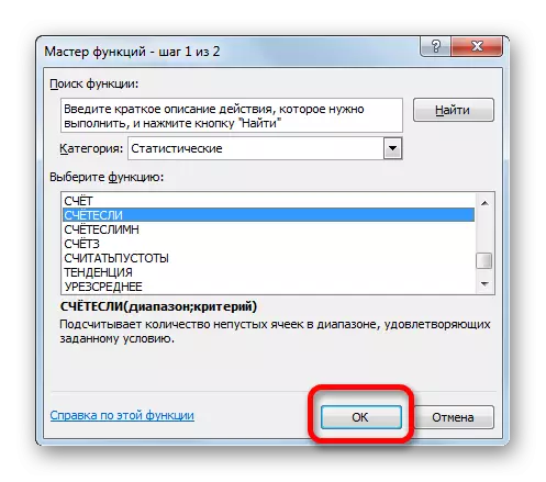
2. Running the wizard of functions. Make moving to the "Statistical" block. There we find and highlight the name "counted". Then should be closed along the "OK" button.



3. Activation of the arguments window of the above operator occurs. In the field "Range", specify the area of ​​the cells, among which will be calculated. In our case, you should select the contents of the Store 2 line, in which the revenues are located by day. We put the cursor to the specified field and, holding the left mouse button, select the appropriate array in the table. The address of the selected array will appear in the window.

   In the next field, the "criterion" just need to specify the immediate selection parameter. In our case, you need to calculate only those elements of the table in which the value exceeds 15000. Therefore, using the keyboard, we drive in the specified field "> 15000" expression.

   After all the above manipulations are manufactured, clay on the "OK" button.



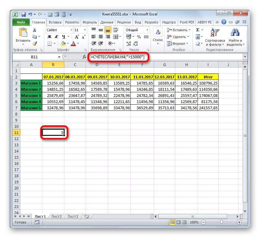
4. The program is calculated and displays the result to the sheet element, which was allocated before activating the functions wizard. As you can see, in this case, the result is equal to the number 5. This means that in the highlighted array in five cells there are values ​​exceeding 15000. That is, it can be concluded that in the store 2 in five days from the analyzed seven revenues exceeded 15,000 rubles.

Lesson: Master of Functions in Excel Program

Countable

The next function that operates the criteria is countable. It also refers to the statistical group of operators. The task of the counsel is counting the cells in the specified array that satisfies a certain set of conditions. It is exactly the fact that you can specify not one, but several parameters, and distinguishes this operator from the previous one. The syntax is as follows:

= Countable (range_longs1; condition1; range_longs2; condition2; ...)

"Condition range" is an identical first argument of the previous operator. That is, it is a reference to the area in which cell counts satisfying the specified conditions will be calculated. This operator allows you to set several such areas at once.

"Condition" is a criterion that determines which elements from the corresponding array of data will include counting, and which will not be included. Each given data area must be specified separately, even if it coincides. It is required that all the arrays used as the conditions of the condition have the same number of rows and columns.

In order to set several parameters of the same data area, for example, to calculate the number of cells in which the values ​​are located more than a certain number, but less than another number, it follows as the argument "Conditions" several times to specify the same array . But at the same time, different criteria should be specified as the corresponding arguments.

On the example, the entire same table with the weekly revenue of the stores will see how it works. We need to know the number of days of the week when income in all these outlets reached the norm established for them. Revenue rates are as follows:

• Shop 1 - 14000 rubles;
• Shop 2 - 15000 rubles;
• Shop 3 - 24000 rubles;
• Shop 4 - 11000 rubles;
• Shop 5 - 32000 rubles.

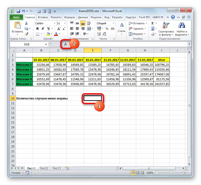
1. To perform the above task, we highlight the cursor an element of the working sheet, where the result is the result of data processing countersmith. Clay on the "Insert function" icon.



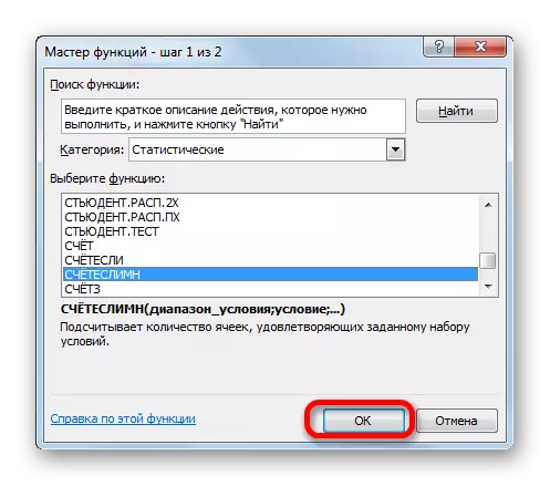
2. Going to the Master of Functions, again move to the "Statistical" block. In the list, it is necessary to find the name of the counting method and produce its allocation. After executing the specified action, you need to press the "OK" button.



3. Following the implementation of the above algorithm of actions, the arguments window opens the countable arguments.

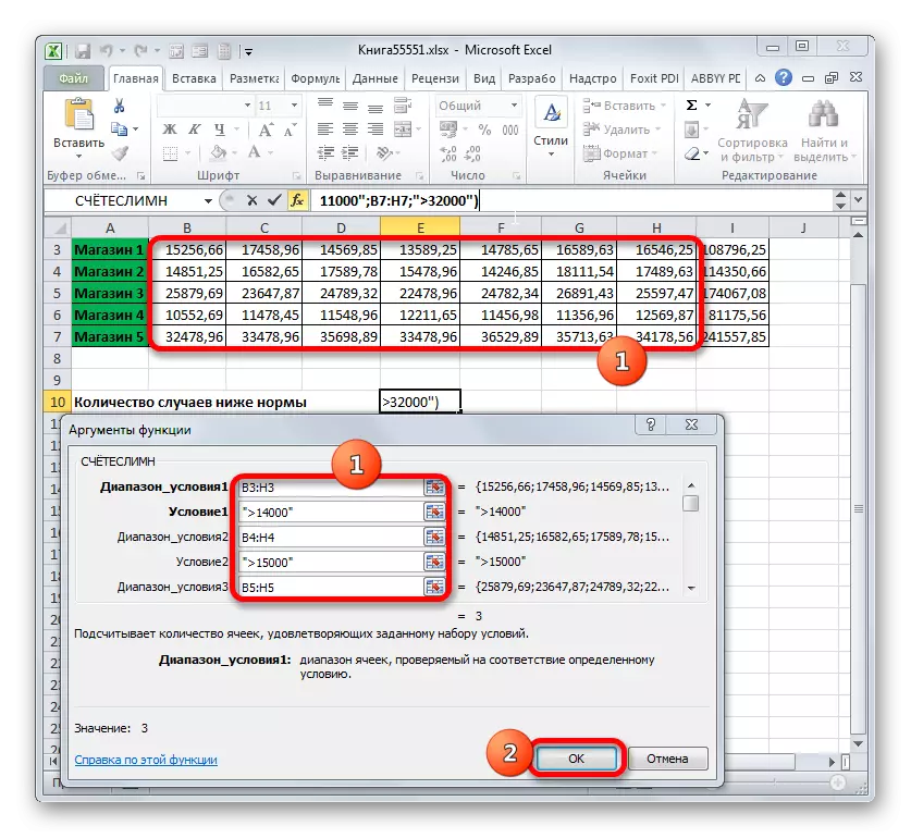
   In the "Condition range" field, enter the address of the string in which the data of the store revenue 1 per week is located. To do this, put the cursor in the field and select the corresponding string in the table. The coordinates are displayed in the window.

   Given that for the store 1, the daily rate of revenue is 14,000 rubles, then in the field "Condition 1" enter the expression "> 14000".

   In the field "Conditions range (3,4,5)" fields, the coordinates of the rows with a weekly revenue of the store 2, store 3, store 4 and store 5. The action is performed by the same algorithm as for the first argument of this group.

   In the field "Condition2", "Condition3", "Condition4" and "Condition5" we introduce the values ​​of "> 15000", "> 24000", "> 11000" and "> 32000". As it is not difficult to guess, these values ​​correspond to the revenue interval exceeding the norm for the corresponding store.

   After all the necessary data was entered (only 10 fields), press the "OK" button.



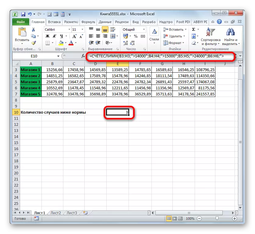
4. The program is calculated and displays the result on the screen. As you can see, it is equal to the number 3. This means that in three days from the analyzed week, revenues in all outlets exceeded the norm established for them.

Now we will change the task somewhat. We should count the number of days in which the store 1 received a revenue exceeding 14,000 rubles, but less than 17,000 rubles.

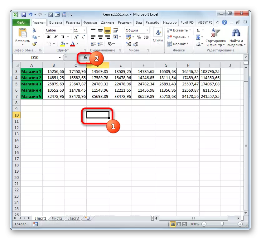
1. We put the cursor to the element where the output is displayed on the counting results sheet. Clay on the "Insert function" icon above the leaf work area.



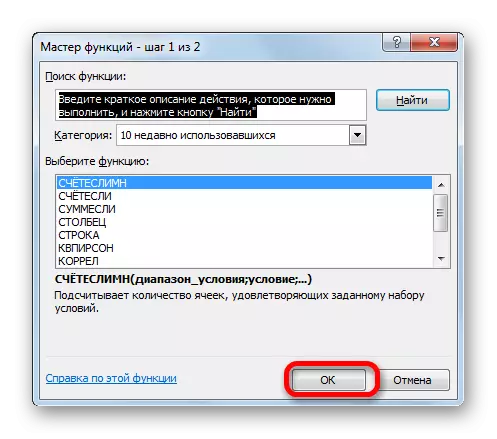
2. Since we have quite recently used the formula of the counting method, now it is not necessary to switch to the "Statistical" group of functions. The name of this operator can be found in the "10 recently used" category. We highlight it and click on the "OK" button.



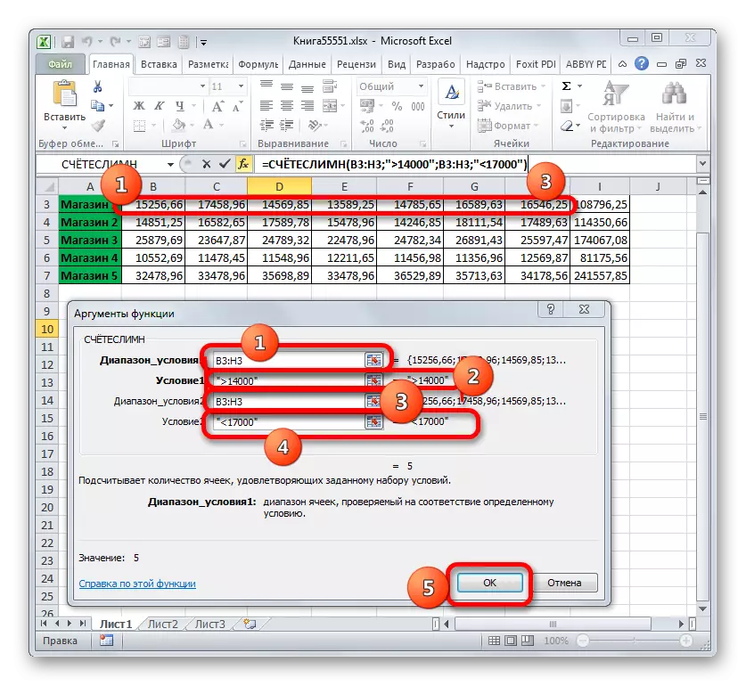
3. An already familiar window of the arguments of the operator counsels opened. We put the cursor in the "Condition range" field and, by selling the left mouse button, select all the cells in which the revenue of the shop is contained 1. They are located in the line, which is called "Store 1". After that, the coordinates of the specified area will be reflected in the window.

   Next, set the cursor in the "Condition1" field. Here we need to specify the lower border of the values ​​in the cells that will take part in the counting. Indicate the expression "> 14000".

   In the field "Conditions2" field, we enter the same address in the same method that was entered in the field "Condition range" field, that is, again we introduce the coordinates of the cells with revenue values ​​on the first outlet.

   In the field "Condition2" indicate the upper limit of the selection: "

   After all these actions are manufactured, we are clay on the "OK" button.



4. The program issues the result of the calculation. As we can see, the final value is 5. This means that in 5 days from the studied seven revenues in the first store was in the range from 14,000 to 17,000 rubles.

Smerei

Another operator that uses the criteria is silent. In contrast to previous functions, it refers to the mathematical block of the operators. Its task is to summarize data in cells that correspond to a specific condition. The syntax is:

= Silent (range; criterion; [Range_Suming])

The "Range" argument indicates the area of ​​the cells that will be checked for compliance with the condition. In fact, it is given by the same principle as the same argument of the function of the function.

"Criterion" is a mandatory argument specifying the selection parameter of the cells from the specified data area that will be summed up. The principles of instructions are the same as that of similar arguments of previous operators, which were considered above.

The "summation range" is an optional argument. It indicates a specific area of ​​the array in which summation will be made. If it is omitted and not specified, then by default it is believed that it is equal to the value of the mandatory argument "Range".

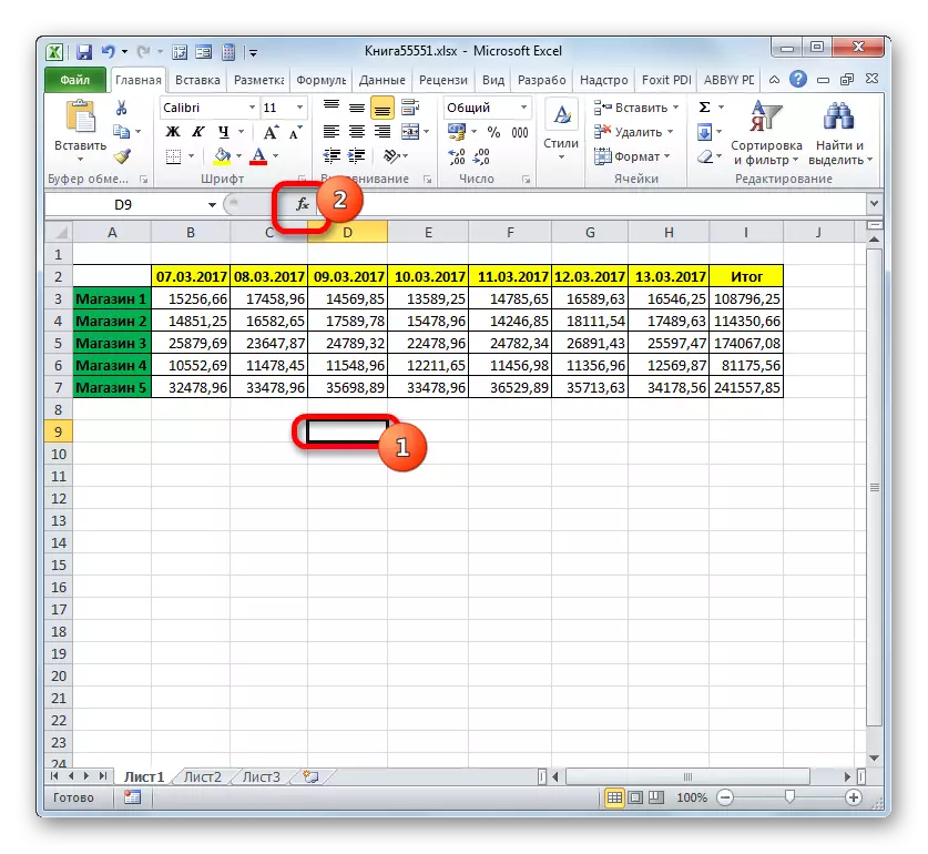
Now, as always, consider the application of this operator in practice. Based on the same table, we are faced with the task to calculate the amount of revenues in the store 1 for the period, starting from 03/11/2017.

1. Select the cell in which the output will be displayed. Click on the "Insert function" icon.



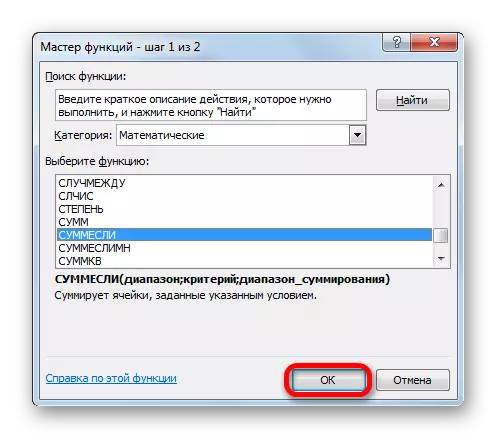
2. Going to the Master of Functions in the "Mathematical" block, we find and highlight the name "silent". Clay on the "OK" button.



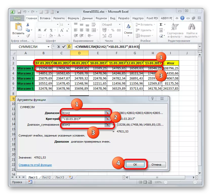
3. The function arguments window will be launched. It has three fields corresponding to the arguments of the specified operator.

   In the "Range" field, we enter the table area in which the values ​​that are checked for compliance with the conditions will be located. In our case, it will be a dates line. We put the cursor in this field and allocate all the cells in which the dates are contained.

   Since we need to fold only the amounts of revenue, starting from March 11, then in the field "Criterion" we drive "> 10.03.2017".

   In the "Summation Range" field, you need to specify the area whose values ​​that meet the specified criteria will be summed up. In our case, these are the values ​​of the revenue of the Store1 line. Select the corresponding array of sheet elements.

   After the introduction of all these data is performed, click on the "OK" button.



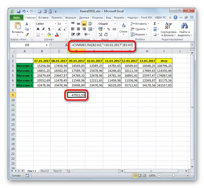
4. After that, the pre-specified element of the working sheet will be displayed the result of data processing function is silent. In our case, it is equal to 47921.53. This means that starting from 11.03.2017, and until the end of the analyzed period, the overall revenue of the store 1 was 47921.53 rubles.

Smemelimn

We completed the study of operators that use the criteria by staying on the functions of Smembremlin. The task of this mathematical function is to summarize the values ​​of the specified table areas selected by several parameters. The syntax of the specified operator is as follows:

= Smerevymn (range of summation; range_longs1; condition1; range_longs2; condition2; ...)

The "summation range" is an argument that is an address of that array, the cells in which corresponding to a certain criterion will be folded.

"Condition range" - an argument representing an array of data verifiable for compliance;

"Condition" is an argument, which is an extraction criterion for addition.

This function implies operations at once with several sets of similar operators.

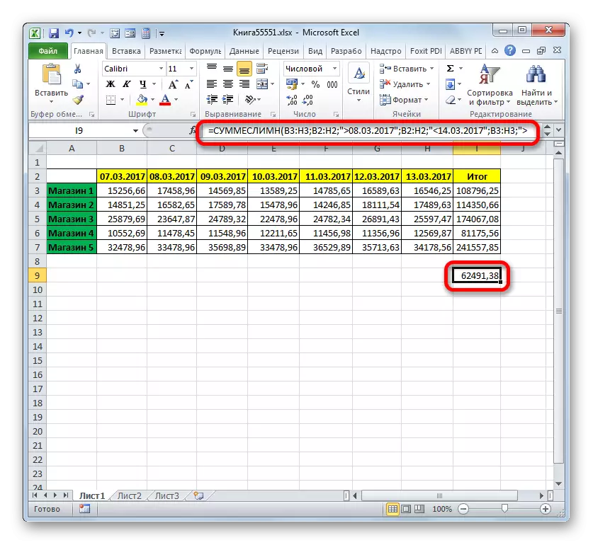
Let's see how this operator is applicable to solving tasks in the context of our revenue table from sales in retail outlets. We will need to calculate the income that the store brought 1 for the period from 09 to 13 March 2017. At the same time, when the income is summarized, only those days in which the revenues exceeded 14,000 rubles should be taken into account.

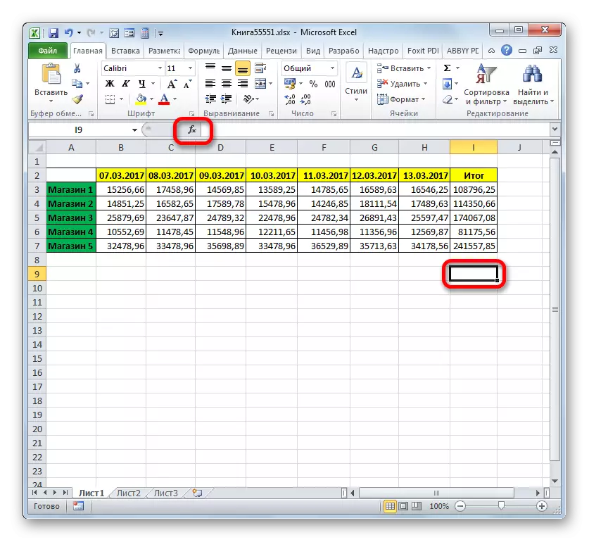
1. Again, select the cell for the output and clay on the "Insert function" icon.



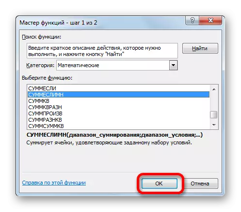
2. In the wizard of functions, first of all, we perform moving to the "mathematical" block, and there we allocate the item called "Smerembremn". We make click on the "OK" button.



3. The operator arguments window starts, the name of which was indicated above.

   Install the cursor in the field of summation range. Unlike subsequent arguments, this one of its kind and points to that array of values ​​where the summation of the data encountered under the indicated criteria will be made. Then select the Store1 line area, in which the revenue values ​​are placed on the corresponding trading point.

   After the address is displayed in the window, go to the "Condition range" field. Here we will need to display the coordinates of the string with dates. We produce clamp left mouse button and highlight all dates in the table.

   We put the cursor in the "Condition1" field. The first condition is that we will be summarized the data not earlier than March 09. Therefore, we enter the value "> 03/03/2017".

   Move to the argument "Conditions Range". Here it is necessary to make the same coordinates that were recorded in the "Condition range" field. We do this in the same way, that is, by allocating a line with dates.

   Install the cursor in the "Condition2" field. The second condition is that the days for which revenue will be summarized should be no later than March 13. Therefore, write down the following expression: "

   Go to the field "Conditions 2" field. In this case, we need to highlight the same array, the address of which was made as an array of summation.

   After the address of the specified array appears in the window, go to the field "Condition3". Given that only values ​​will take part in summation, whose value exceeds 14,000 rubles, introduce the record of the following nature: "> 14000".

   After the last action is performed by clay on the "OK" button.



4. The program displays the result on the sheet. It is equal to 62491.38. This means that for the period from 09 to 13 March 2017, the amount of revenue when it is additioned for the days in which it exceeds 14,000 rubles, amounted to 62491.38 rubles.

Conditional formatting

The latter, described by us, tool, when working with which criteria are used, is conditional formatting. It performs the specified formatting type of cells that meet the specified conditions. Look at an example of working with conditional formatting.

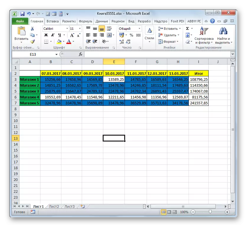
We highlight those cells of the table in blue, where values ​​per day exceed 14,000 rubles.

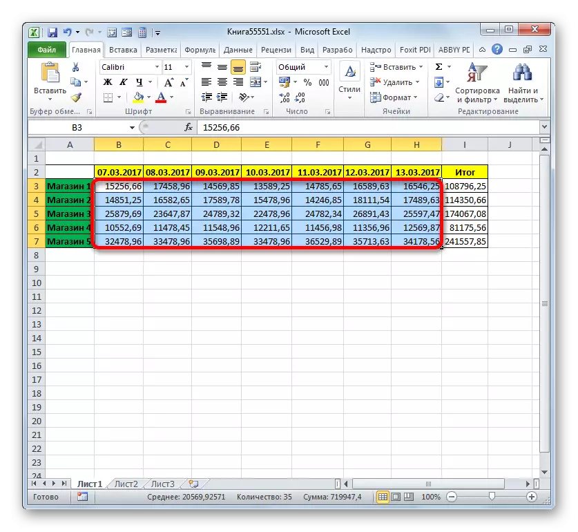
1. We allocate the entire array of elements in the table, which indicates the revenue of the outlets by day.



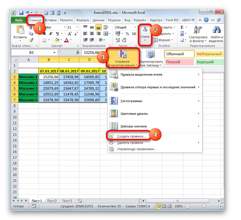
2. Moving to the "Home" tab. Clay on the "Conditional Formatting" icon placed in the "Styles" block on the tape. A list of actions opens. We put on it on the position "Create a rule ...".



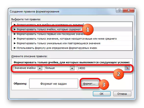
3. The formatting rule generation is activated. In the field selection area, we allocate the name "format only cells that contain". In the first field of the block of conditions from the list of possible options, select "Cell value". In the next field, choose the "more" position. In the latter, we specify the value itself, the larger of which is required to format the elements of the table. We have 14,000. To select the type of formatting, clay on the "Format ..." button.



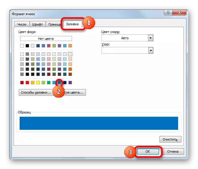
4. The formatting window is activated. Moving to the "Fill" tab. From the proposed colors of the pouring colors, select blue by clicking on it with the left mouse button. After the selected color appeared in the "Sample" area, clay on the "OK" button.



5. Automatically returns to the formatting rule generation. In it, both blue color is displayed in the sample area. Here we need to produce one single action: to be placed on the "OK" button.



6. After completing the last action, all cells of the highlighted array, where the number is contained greater than 14000, will be filled with blue.

In more detail about the possibilities of conditional formatting, it is described in a separate article.

Lesson: Conditional formatting in the Excel program

As you can see, with the help of tools using criteria when working, it is possible to solve quite diverse tasks in Excele. It can be like counting amounts and values ​​and formatting, as well as the execution of many other tasks. The main tools running in this program with criteria, that is, with certain conditions, when executing which the specified action is activated, is a set of built-in functions, as well as conditional formatting.