Excel difference formula: 4 simple ways

The calculation of the difference is one of the most popular actions in mathematics. But this calculation is applied not only in science. We constantly perform it, without even thinking, and in everyday life. For example, in order to calculate the delivery of the purchase in the store, it is also used to calculate the difference between the amount that the buyer gave the seller, and the cost of goods. Let's see how to calculate the difference in Excel when using various data formats.

Calculation of difference

Considering that Excel works with various data formats, when subtracting one value from another, various formula variants are used. But in general, everything can be reduced to a single type:

X = a-b

And now let's look at how the values ​​of various formats are subtracted: numerical, money, dates and time.

Method 1: Subtract numbers

Immediately let's consider the most commonly applicable variant of the calculation of the difference, namely the subtraction of numeric values. For these purposes, an ordinary mathematical formula with a sign "-" can be applied in Excele.

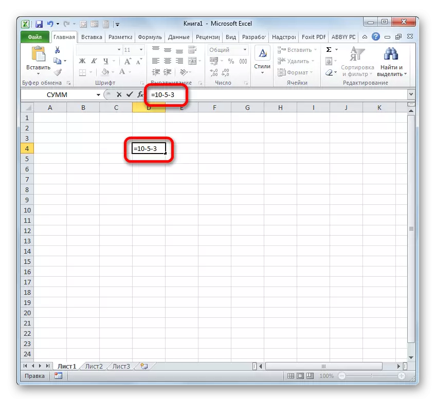
1. If you need to make the usual subtraction of numbers by using Excel, as a calculator, then set the "=" symbol in the cell. Then immediately after this symbol, a decreased number from the keyboard should be recorded, put the symbol "-", and then record the subtracted one. If you are deducted somewhat, then you need to put the "-" symbol again and record the desired number. The procedure for the alternation of a mathematical sign and numbers should be carried out until all subtracts are entered. For example, from among the 10 subtract 5 and 3, you need to write the following formula to the Excel sheet element:

   = 10-5-3.

   After writing an expression, to derive the result of the counting, click on the Enter key.



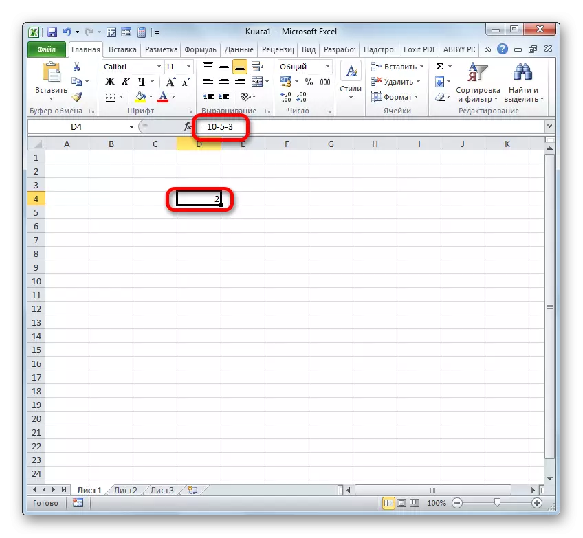
2. As you can see, the result appeared. It is equal to number 2.

But significantly more often the subtraction process in Excel is used between the numbers placed in the cells. At the same time, the algorithm of mathematical action is practically not changed, only now instead of specific numerical expressions, links to cells are used, where they are located. The result is displayed in a separate element of the sheet, where the character "=" is installed.

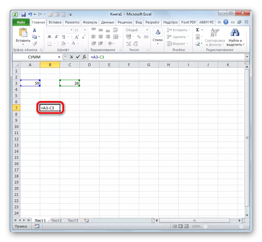
Let's see how to calculate the difference between numbers 59 and 26, located respectively in the elements of the sheet with the coordinates of A3 and C3.

1. Select an empty element of the book in which we plan to display the result of the calculation of the difference. We put in it the symbol "=". After that, click on the cell A3. We put the symbol "-". Next, we perform click on the element of the C3 sheet. The following form should appear in the sheet element for the output of the result:

   = A3-C3

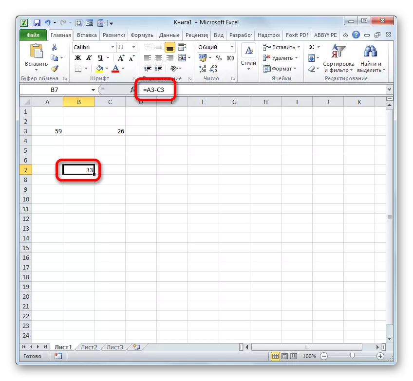
   As in the previous case, to display the result on the screen, click the Enter key.



2. As we see, in this case the calculation was performed successfully. The counting result is equal to the number 33.

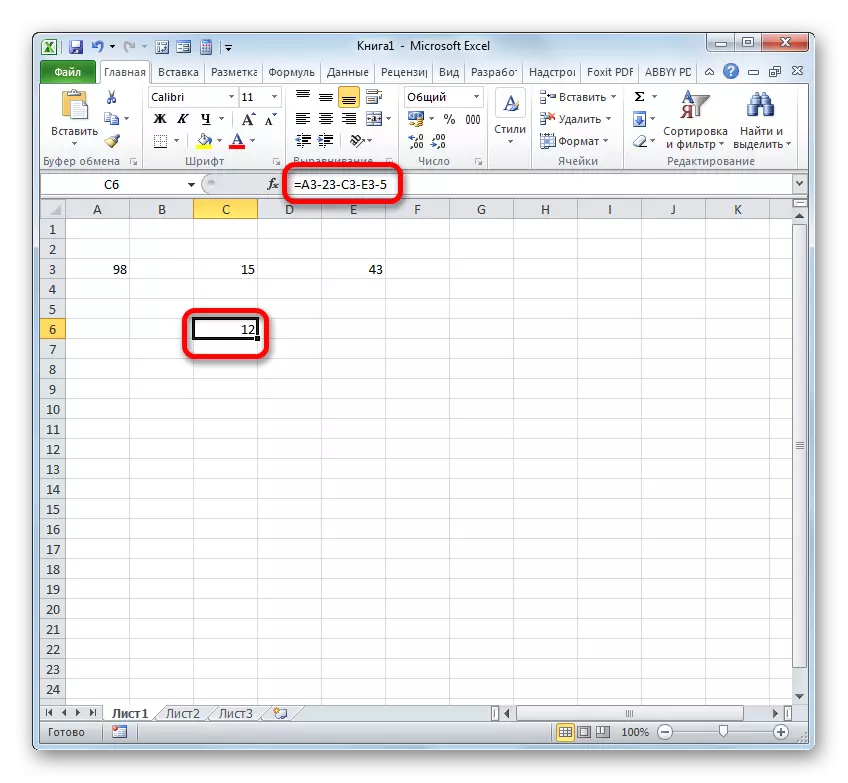
But in fact, in some cases, it is necessary to make a subtraction in which they will take part, both directly numerical values ​​and links to cells where they are located. Therefore, the expression, for example, as follows:

= A3-23-C3-E3-5

Lesson: How to subtract the number from among the exale

Method 2: cash format

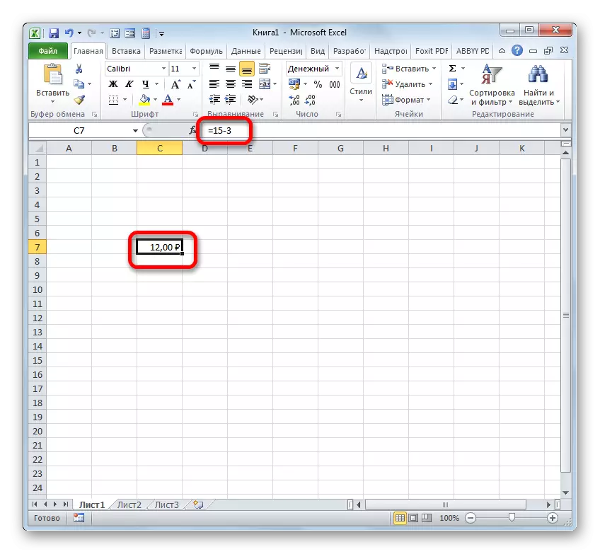
The calculation of the values ​​in cash format is practically no different from numerical. The same techniques are used, since, by and large, this format is one of the numerical options. The difference is only that at the end of the values ​​participating in the calculations, a monetary symbol of a particular currency is established.

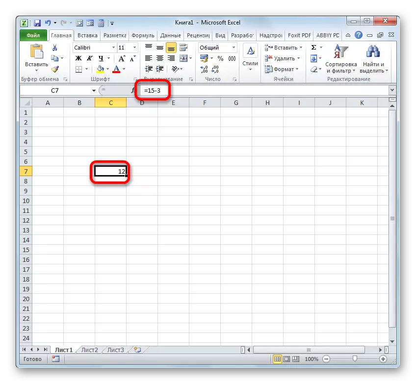
1. Actually, you can conduct an operation as the usual subtraction of numbers, and only then format the final result for a cash format. So, we produce a calculation. For example, will subtract out of the 15th number 3.



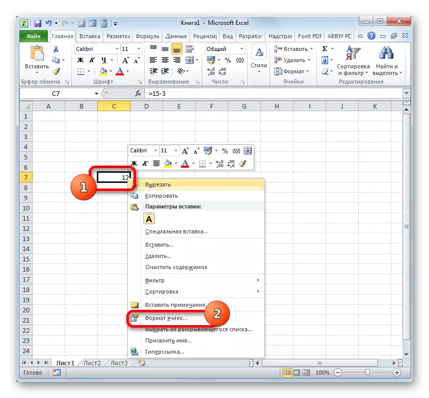
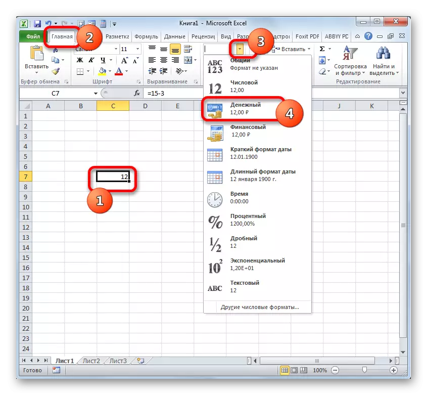
2. After that, click on the sheet item, which contains the result. In the menu, select the value of the "cell format ...". Instead of calling the context menu, you can apply after the selection of the Ctrl + 1 keys.



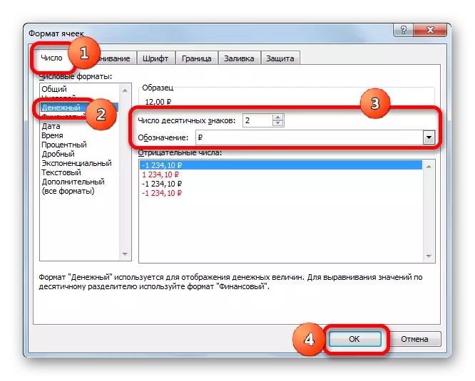
3. With any of the two specified options, the formatting window is launched. Move into the "Number" section. In the "Numeric formats" group it should be noted the "money" option. At the same time, special fields will appear on the right side of the window interface, in which you can choose a currency type and the number of decimal signs. If you have Windows as a whole and Microsoft Office, in particular, localized for Russia, then by default there should be a ruble symbol, and in the field of decimal signs, the number "2". In the overwhelming majority of cases, these settings are not needed. But, if you still need to make calculation in dollars or without decimal signs, it is required to make the necessary adjustments.

   Following how all the necessary changes are made, clay on "OK".



4. As we can see, the result of subtraction in the cell was transformed into a cash format with a set number of decimal signs.

There is another option to format the resulting subtracting for a cash format. To do this, you need to click on the Ribbon in the "Home" tab on the triangle located on the right of the display field of the current cell format in the "Number" toolbar. From the opening list, select the "money" option. Numeric values ​​will be converted into cash. True, in this case, there is no possibility of choosing a currency and the number of decimal signs. A variant that is set in the default system, or is configured via the formatting window described by us above.

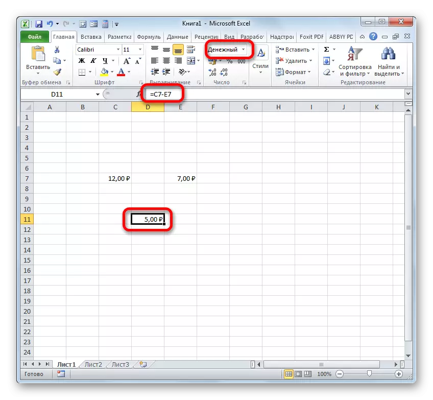
If you calculate the difference between the values ​​in the cells that are already formatted for a cash format, then format the leaf element for the output of the result is not even necessary. It will be automatically formatted under the appropriate format after the formula is entered with links to elements containing the reduced and subtracted numbers, as well as a click on the Enter key.

Lesson: How to change cell format in Excel

Method 3: Dates

But the calculation of the dates difference has essential nuances other than previous options.

1. If we need to subtract a certain number of days from the date specified in one of the elements on the sheet, then first of all set the "=" symbol into the item where the final result will be displayed. After that, click on the sheet item, where the date contains. Its address will be displayed in the output element and in the formula string. Next, we set the symbol "-" and drive the number of days from the keyboard that you need to take away. In order to calculate the clay on Enter.



2. The result is displayed in the cell designated by us. In this case, its format is automatically converted into the date format. Thus, we get a full-fledged date.

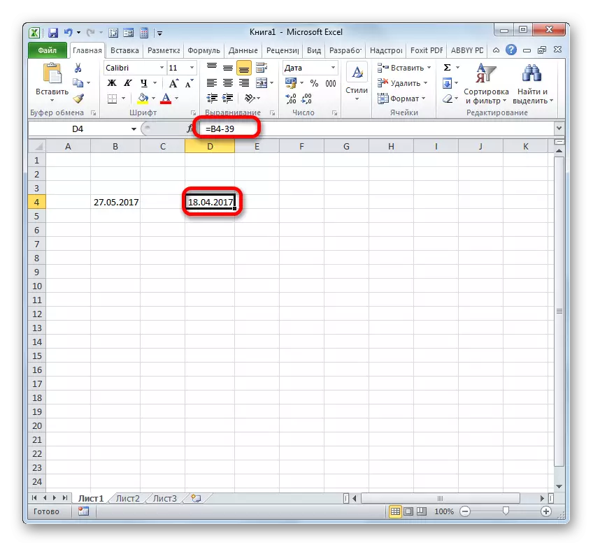
There is also an inverse situation when it is required from one date to subtract another and determine the difference between them in days.

1. Install the character "=" into the cell where the result will be displayed. After that, we have a clay on the element of the sheet, where the later date is contained. After its address appeared in the formula, we set the symbol "-". Clay in a cell containing an early date. Then clay on ENTER.



2. As you can see, the program accurately calculated the number of days between the specified dates.

Also, the difference between dates can be calculated using the solution function. It is good because it allows you to configure with the help of an additional argument, in which units of measurement will be derived a difference: months, days, etc. The disadvantage of this method is that work with functions is still more difficult than with conventional formulas. In addition, the solute operator is missing in the list of functions wizard, and therefore it will have to be administered manually by applying the following syntax:

= Commands (Nach_Data; Kon_DAT;

The "initial date" is an argument, which is an early date or reference to it, located in the element on the sheet.

The "final date" is an argument in the form of a later date or link to it.

The most interesting argument "one". With it, you can choose the option exactly how the result will be displayed. It can be adjusted using the following values:

• "D" - the result is displayed in days;
• "M" - in full months;
• "Y" - in full years;
• "YD" - a difference in days (excluding years);
• "MD" is a difference in days (excluding months and years);
• "YM" is the difference in months.

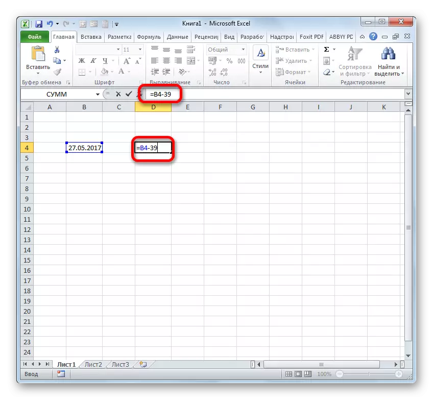
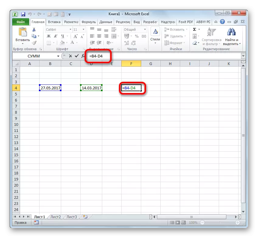
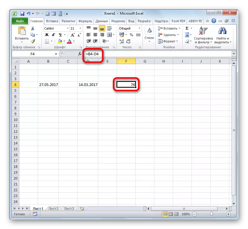
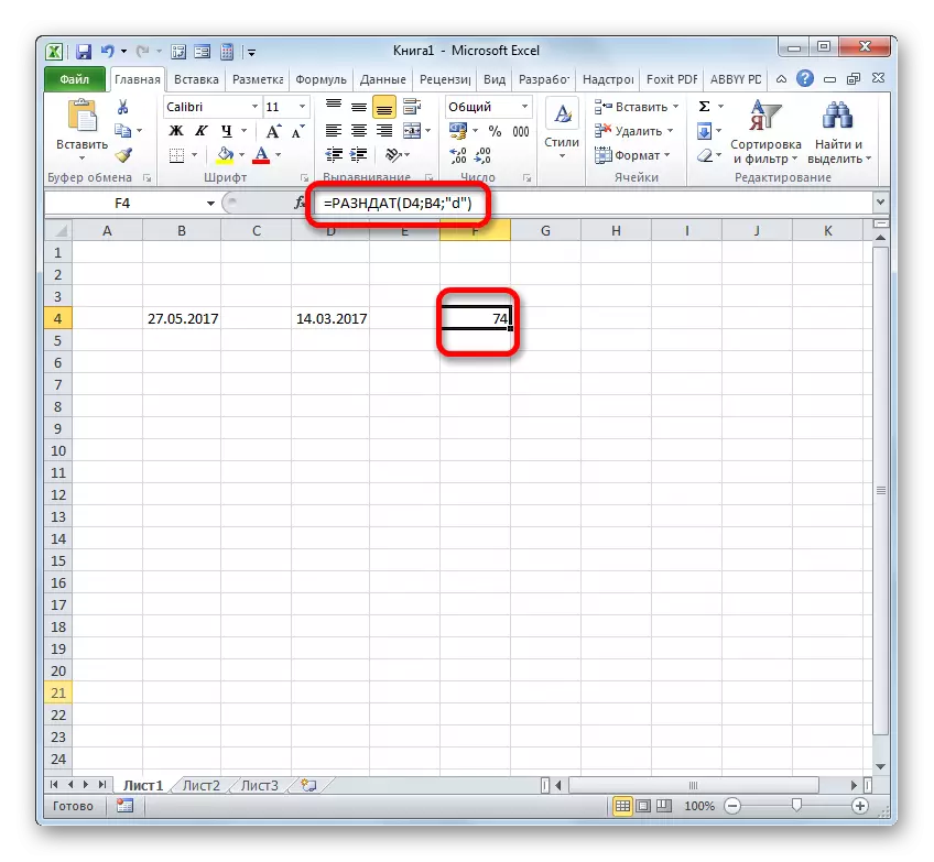
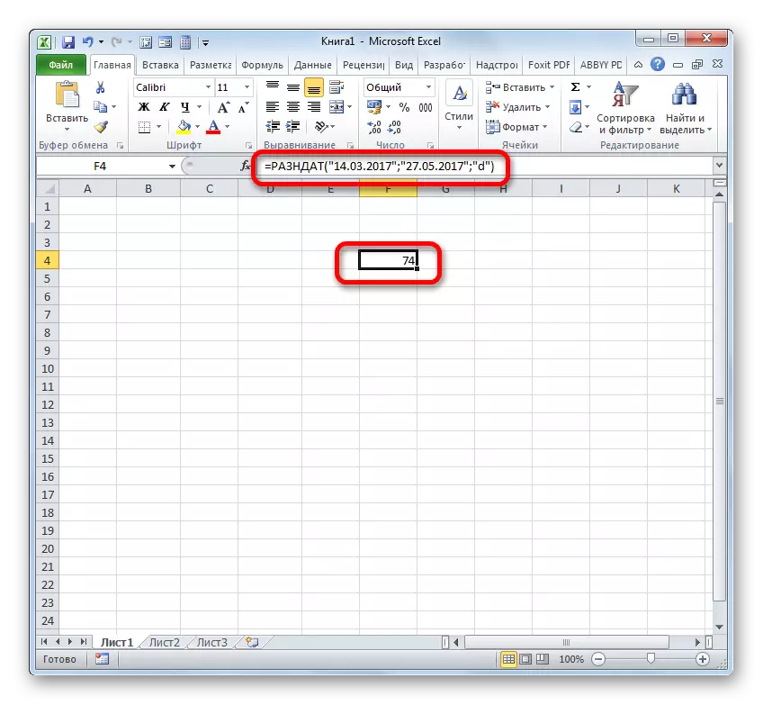
So, in our case, it is necessary to calculate the difference in days between May 27 and March 14, 2017. These dates are located in cells with coordinates B4 and D4, respectively. We establish the cursor in any empty sheet element, where we want to see the results of the calculation, and write down the following formula:

= D4; B4; "D")

We click on ENTER and get the final result of the calculation of the difference 74. Indeed, between these dates lies 74 days.

If it is necessary to deduct the same dates, but without entering them into the cells of the sheet, then in this case we use the following formula:

= Ottes ("03/14/2017"; "27.05.2017"; "D")

Shake the ENTER button again. As we see, the result is naturally the same, only obtained slightly in another way.

Lesson: Number of days between dates in Excele

Method 4: Time

Now we approached the study of the algorithm for subtracting time in Excele. The main principle remains the same as when subtracting dates. You need to take away early from a later time.

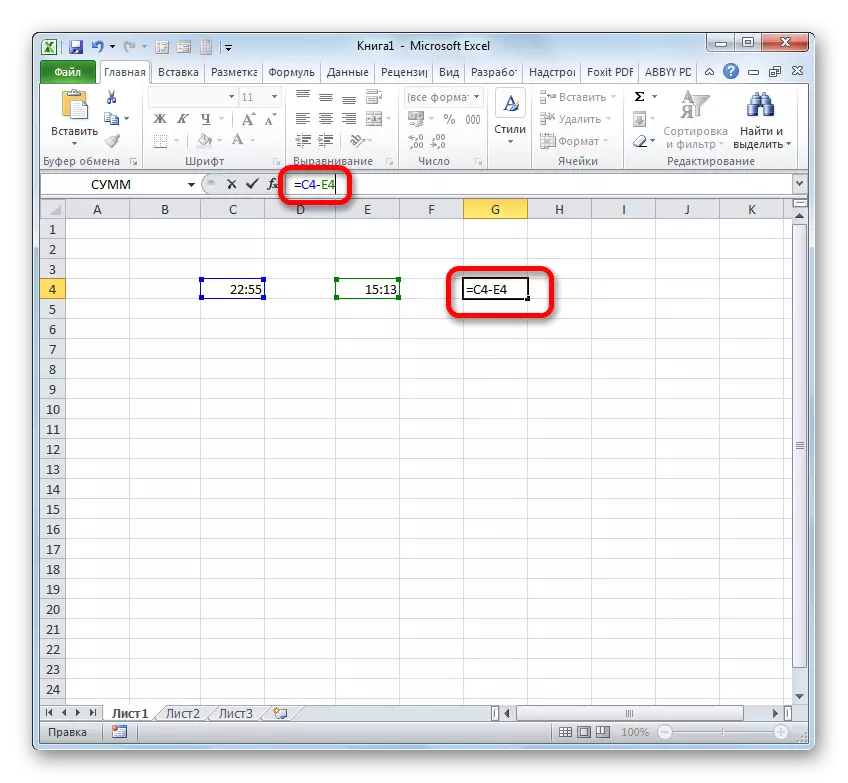
1. So, we are faced with the task of finding how many minutes passed from 15:13 to 22:55. We write these time values ​​into separate cells on the sheet. What is interesting, after entering data, the sheet elements will be automatically formatted under the contents if they have not formatted before. In the opposite case, they will have to format under the date manually. In that cell, in which the result of subtraction will be displayed, we put the character "=". Then we clasme the element containing a later time (22:55). After the address is displayed in the formula, we enter the character "-". Now we are clay on an element on a sheet in which the earliest time is located (15:13). In our case, the formula of the form:

   = C4-E4

   To count clay on ENTER.



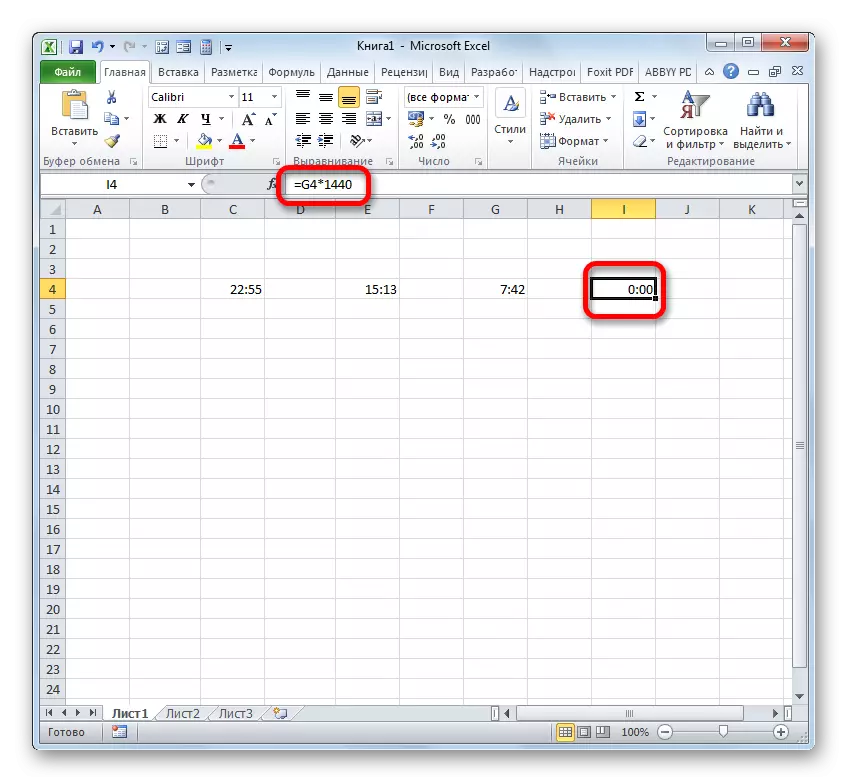
2. But, as we see, the result was displayed a bit not in the form in which we desired. We needed a difference only in minutes, and was displayed 7 hours 42 minutes.

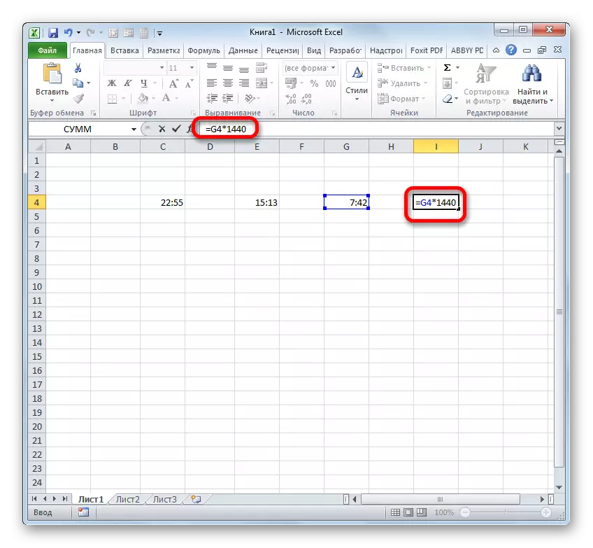
   In order to get a minute, we follow the previous result to multiply by the coefficient 1440. This coefficient is obtained by multiplying the number of minutes in an hour (60) and hours in days (24).

So, set the "=" symbol in an empty cell on the sheet. After that, we produce click on that element of the sheet, where the difference in time subtracting is located (7:42). After the coordinates of this cell were displayed in the formula, click on the "Multiply" symbol (*) on the keyboard, and then you also pick up the number 1440. To obtain the result with clay on ENTER.



3. But, as we see, again the result appeared incorrectly (0:00). This is due to the fact that when multiplying the leaf element was automatically reformatted in the time format. In order to make a difference in minutes, we need to return the general format to it.



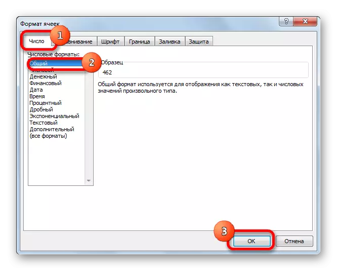
4. So, we allocate this cell and in the "Home" tab by clay on the already familiar triangle to us to the right of the format display field. In the activated list, select the "General" option.

   

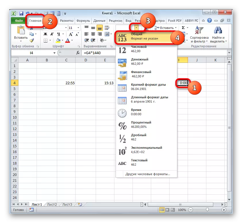
   You can enter differently. Select the specified sheet element and press the Ctrl + 1 keys. The formatting window is launched with which we have already dealt with earlier. Move into the "Number" tab and in the list of numeric formats, select the "General" option. Clay on "OK".



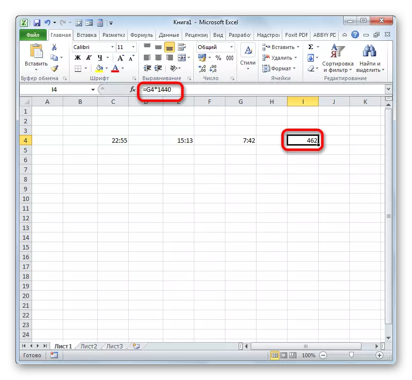
5. After using any of these variants, the cell is reformatted in a general format. It displays the difference between the specified time in minutes. As you can see, the difference between 15:13 and 22:55 is 462 minutes.

Lesson: how to translate the clock in minutes in Excel

As we see, the nuances of counting the difference in Excel depend on how the user works with the data format. But, nevertheless, the general principle of approach to this mathematical action remains unchanged. It is necessary to subtract different from one number. This manages to achieve with mathematical formulas that are applied based on the special Excel syntax, as well as using embedded functions.