How to put a tick in Excele: 5 working ways

In the Microsoft Office program, the user sometimes need to insert a tick or, as a different one is called this element, check box (˅). This can be performed for various purposes: just for the mark of some object, to include various scenarios, etc. Let's find out how to install a tick in Excele.

Installing flag

There are several ways to put a tick in Excel. In order to determine the specific option, you need to immediately install, for which you need to install the checkbox: just for marking or to organize certain processes and scenarios?

Lesson: How to put a tick in Microsoft Word

Method 1: Insert through the menu "Symbol"

If you need to install a tick on visual purposes only to mark some object, you can simply use the "Symbol" button located on the tape.

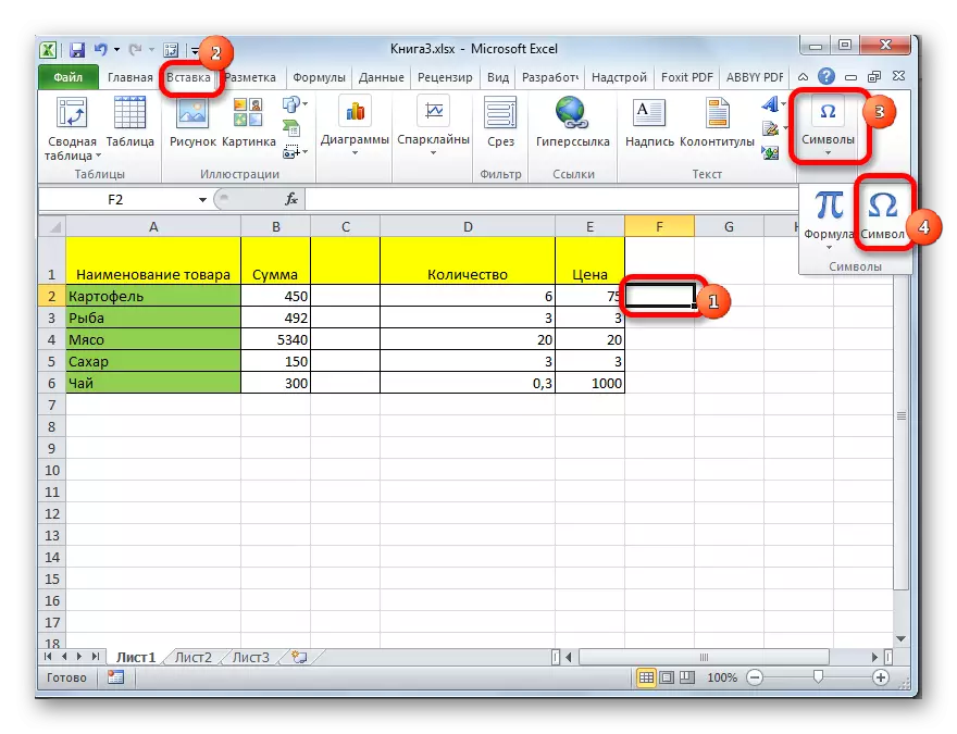
1. Install the cursor in the cell in which the check mark should be located. Go to the "Insert" tab. Click on the "Symbol" button, which is located in the "Symbols" toolbar.



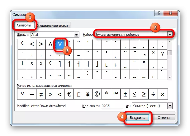
2. A window opens with a huge list of various elements. We do not go anywhere, but remain in the "Symbols" tab. In the Font field, any of the standard fonts can be specified: Arial, Verdana, Times New Roman, etc. To quickly search for the desired symbol in the "Set" field, set the parameter "Letters of gap changes". We are looking for a symbol "˅". We highlight it and click on the "Paste" button.

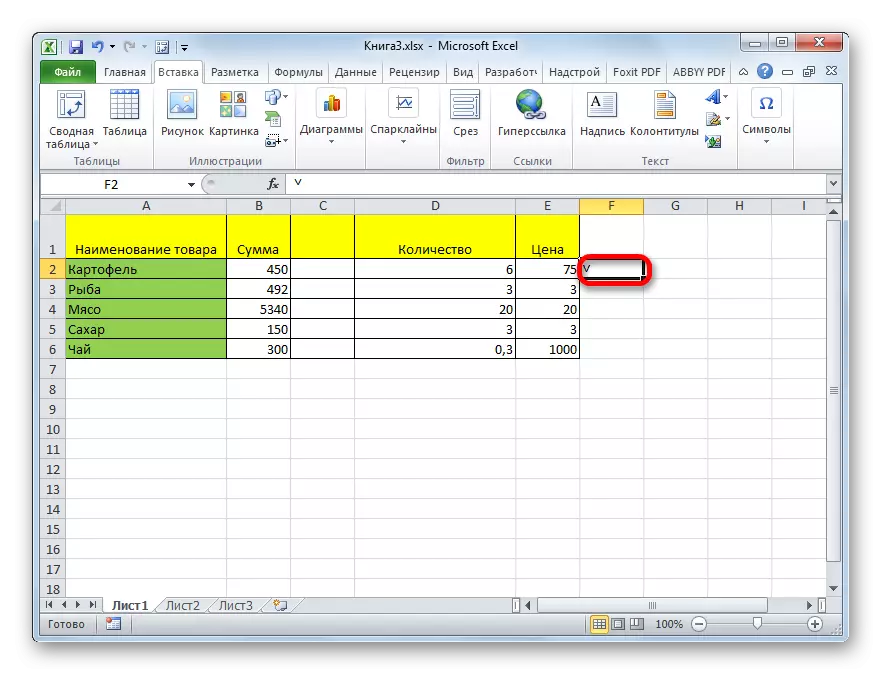
After that, the selected element will appear in the pre-specified cell.

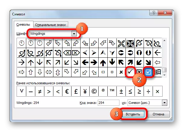
In the same way, you can insert a more familiar tick with disproportionate sides or a check mark in Chexbox (a small square, specially intended for installation of the flag). But for this, you need to specify in the "Font" field instead of the standard option WingDings special feature. Then you should fall at the bottom of the list of characters and select the desired symbol. After that, we click on the "Paste" button.

The selected sign is inserted into the cell.

Method 2: Character Substitution

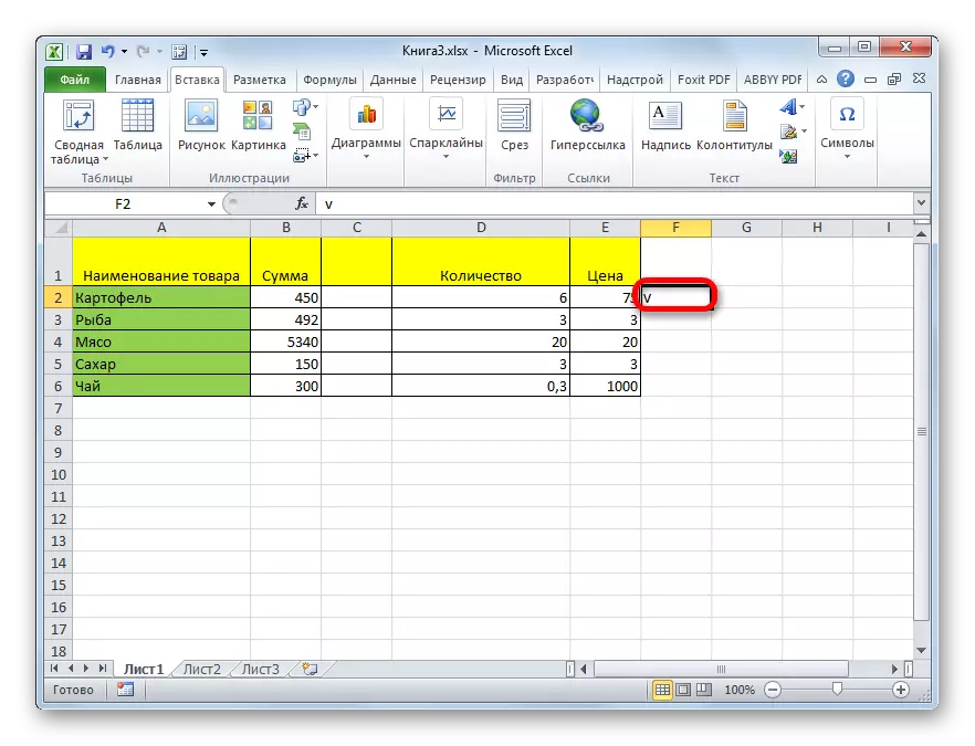
There are also users who are not specified by the exact conformity of characters. Therefore, instead of installing a standard check mark, the "V" symbol in the English-speaking layout is simply printed from the keyboard. Sometimes it is justified, since this process takes very little time. And externally, this substitution is practically invisible.

Method 3: Installation Tick in Chekbox

But in order for the status of the installation or removal of the tick launched some scenarios, you need to perform more difficult operation. First of all, checkbox should be installed. This is such a small square where the checkbox is set. To insert this item, you need to enable the developer menu, which is turned off by default in Excele.

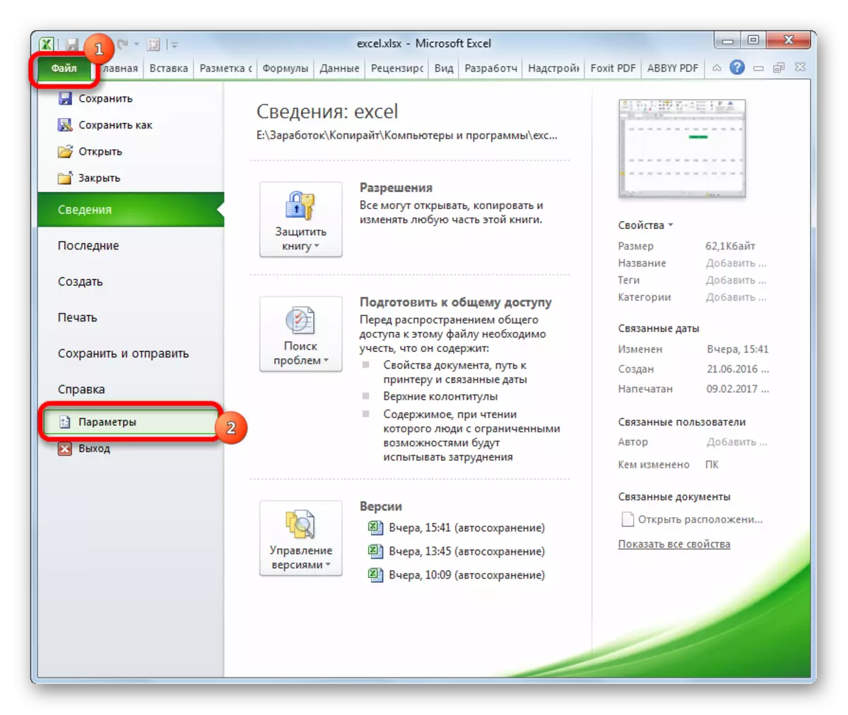
1. Being in the "File" tab, click on the "Parameters" item, which is located on the left side of the current window.



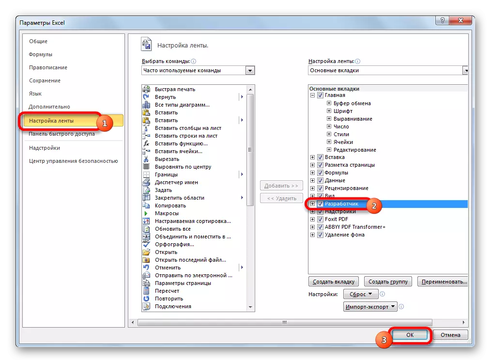
2. The parameter window starts. Go to the "Tape Settings" section. In the right part of the window, we install a tick (it is precisely that we will need to install on the sheet) opposite the "Developer" parameter. At the bottom of the window click on the "OK" button. After that, the Developer tab will appear on the tape.



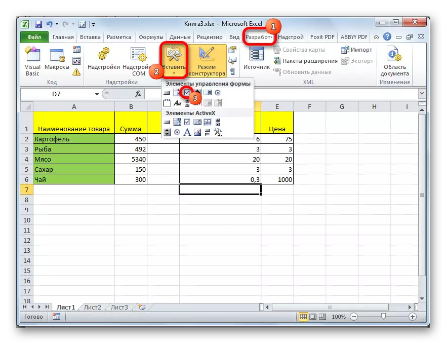
3. Go to the newly activated tab "Developer". In the "Controls" toolbar on the ribbon we click on the "Paste" button. In the list that opens in the "Form Management Elements" group, select "Checkbox".



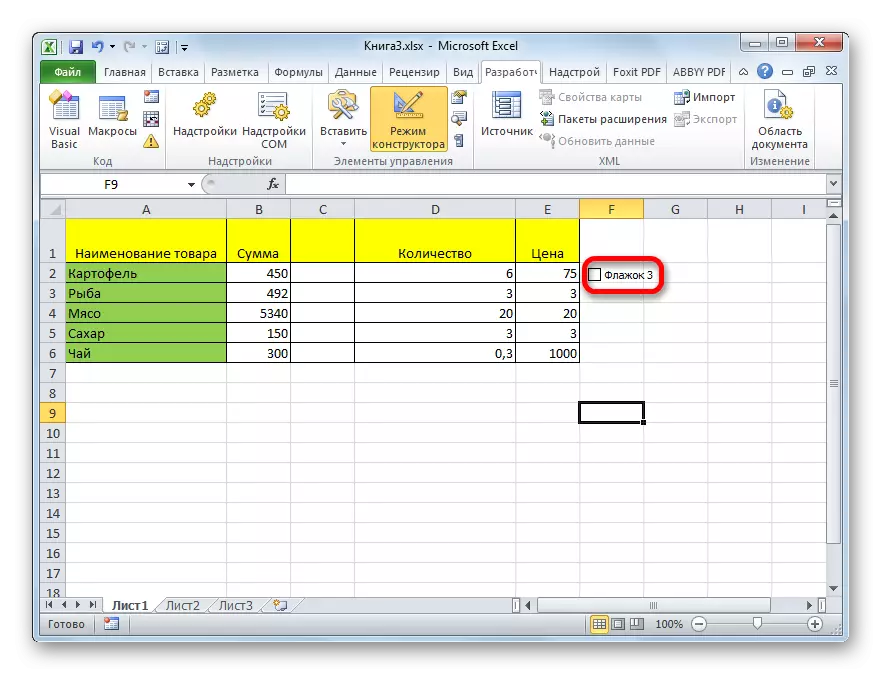
4. After that, the cursor turns into a cross. Click them for the area on the sheet where you need to insert the form.

   

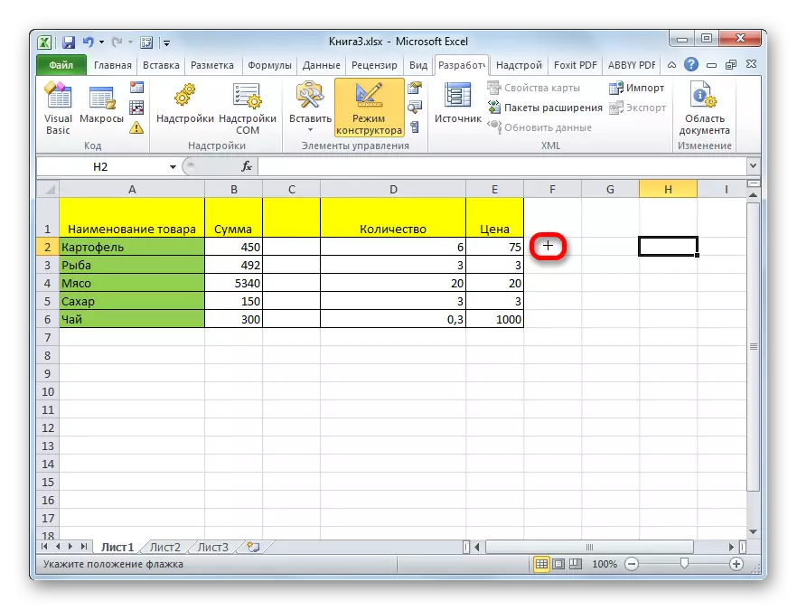
   Empty Chekbox appears.



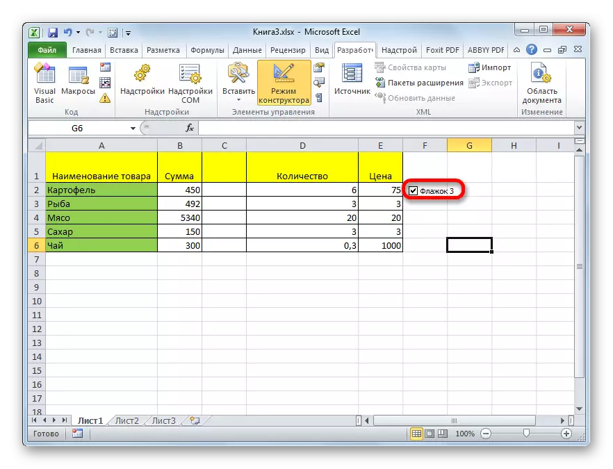
5. To install in it, you need to simply click on this item and the check box will be installed.



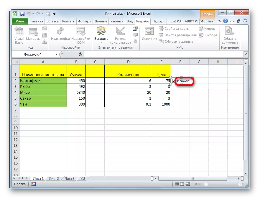
6. In order to remove the standard inscription, which in most cases is not needed by clicking on the left mouse button on the element, select the inscription and press the DELETE button. Instead of remote inscriptions, you can insert another, and you can not insert anything, leaving Chekbox without name. This is at the discretion of the user.



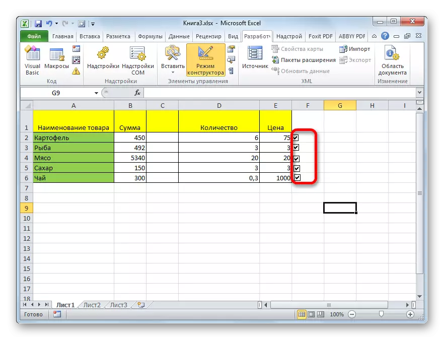
7. If there is a need to create multiple checkboxes, then you can not create a separate one for each row, but to copy it ready, which will significantly save time. To do this, we immediately release the mouse click form, then clamp the left button and drag the form to the desired cell. Do not throw the mouse button, clamp the Ctrl key, and then release the mouse button. We are experiencing a similar operation with other cells in which you need to insert a tick.

Method 4: Creating a Chekbox to perform a script

Above we learned how to put a tick in a cell in various ways. But this feature can be used not only for visual display, but also to solve specific tasks. You can install various scenarios options when switching the checkbox in Chekbox. We will analyze how it works on the example of changing the color of the cell.

1. Create a checkbox in the algorithm described in the previous method using the developer tab.
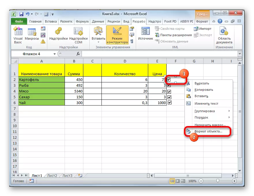
2. Click on the item right-click. In the context menu, select the item "Format of the object ...".



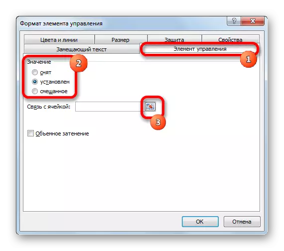
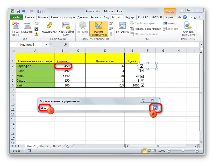
3. The formatting window opens. Go to the "Control" tab, if it was opened elsewhere. In the "Value" parameters, the current state must be specified. That is, if the checkbox is currently installed, the switch must stand in the "set" position, if not, in the position "removed". The "mixed" position is not recommended. After that, we click on the icon near the field "Communication with the cell".



4. The formatting window is folded, and we need to highlight the cell on a sheet with a checkbox with a check mark. After the choice is made, re-press the same button as a pictogram, which was discussed above to return to the formatting window.



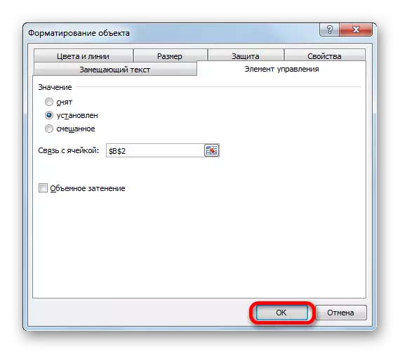
5. In the formatting window, click on the "OK" button in order to save the changes.

   

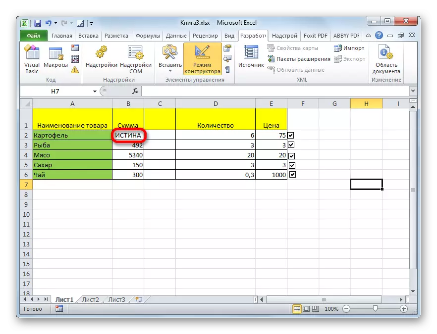
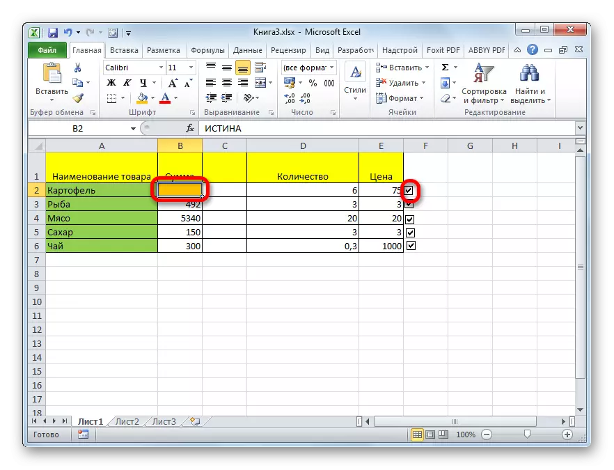
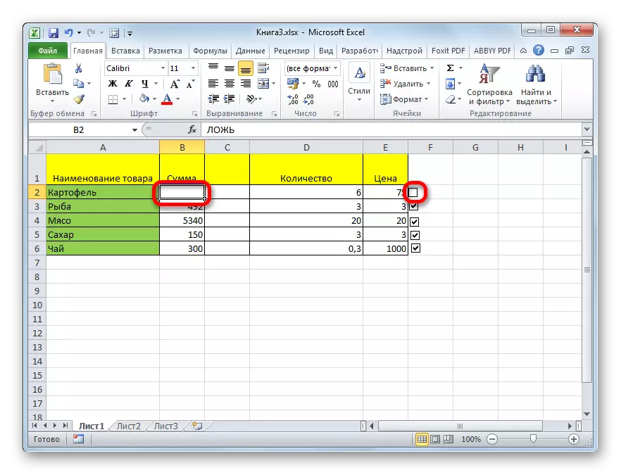
   As you can see, after performing these actions in the associated cell when the checkbox is set in the checkbox, the "Truth" value is displayed. If the tick is removed, then the "Lie" value will be displayed. To fulfill our task, namely, to change the colors of the fill, you will need to link these values ​​in a cell with a specific action.



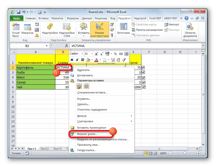
6. We highlight the associated cell and click on it right mouse button, select the "cell format ..." in the opened menu.



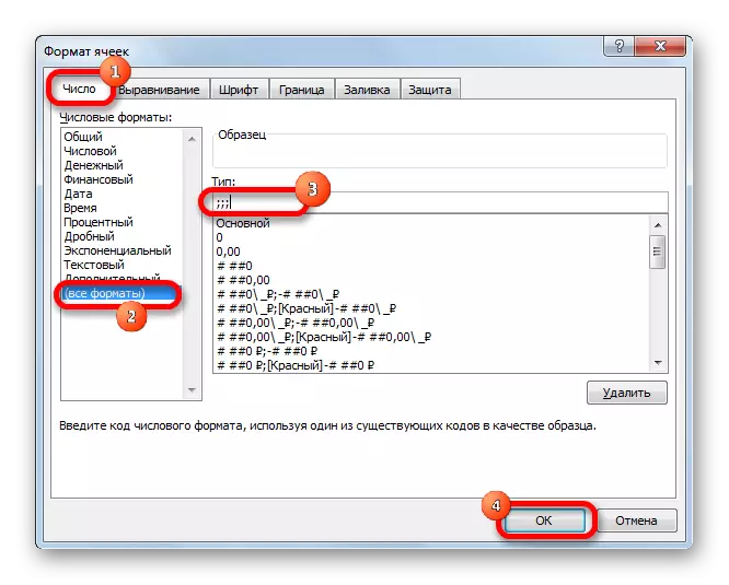
7. Cell formatting window opens. In the "Number" tab, we allocate the "All Formats" item in the "Numeric formats" parameters. The field "Type", which is located in the central part of the window, prescribe the following expression without quotes: ";;; " Click on the "OK" button at the bottom of the window. After these actions, the visible inscription "Truth" from the cell disappeared, but the value remains.



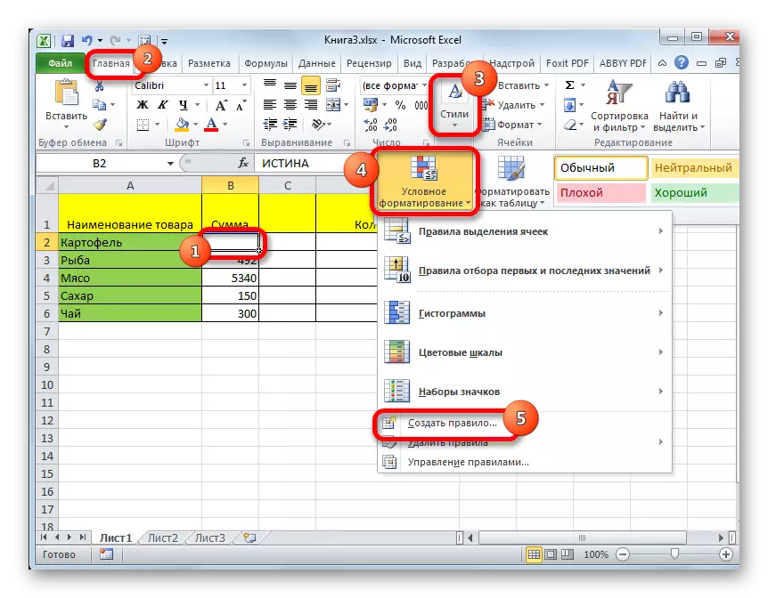
8. We allocate the associated cell and go to the "Home" tab. Click on the "Conditional Formatting" button, which is located in the "Styles" tools block. In the list of clicking on the item "Create a rule ...".



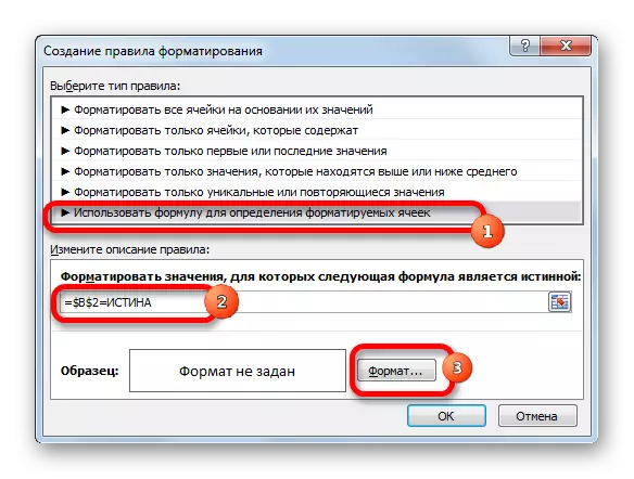
9. The formatting rule creation window opens. In its top you need to choose the type of rule. Select the latest point in the list: "Use the formula to determine the formatable cells." In the "Format the values ​​for which the following formula is true" specify the address of the connected cell (this can be done as manually, and simply allocation of it), and after the coordinates appeared in the line, add the expression "= truth" in it. To set the selection color, click on the "Format ..." button.



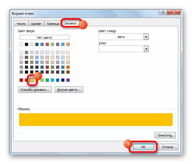
10. Cell formatting window opens. We choose the color that would like to pour the cell when the tick is turned on. Click on the "OK" button.



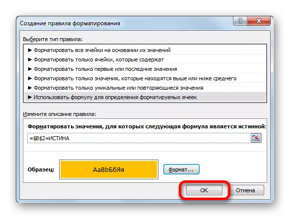
11. Returning to the Create Rules window, click on the "OK" button.

Now, when the checkbox is turned on, the associated cell will be painted in the selected color.

If the checkbox is cleaned, the cell will again become white.

Lesson: Conditional formatting in Excel

Method 5: Installation Tick using ActiveX tools

Tick ​​can also be installed using ActiveX tools. This feature is available only through the developer menu. Therefore, if this tab is not enabled, it should be activated, as described above.

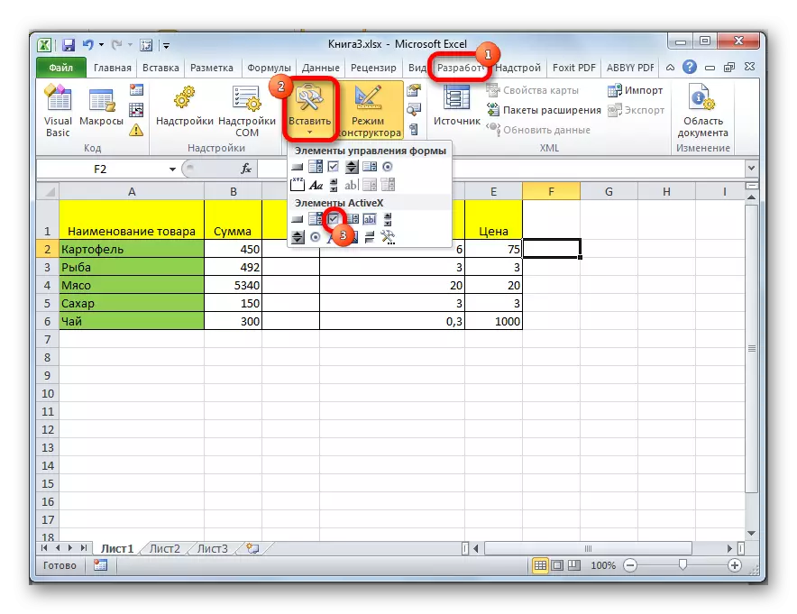
1. Go to the Developer tab. Click on the "Insert" button, which is posted in the "Controls" toolbar. In the window that opens in the ActiveX elements block, select the checkbox.



2. As in the previous time, the cursor takes a special form. We click on them by the place of the sheet, where the form should be placed.



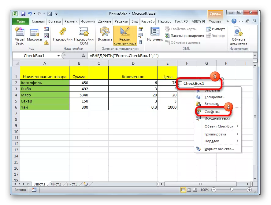
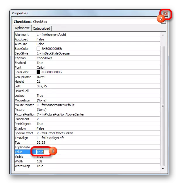
3. To set the check mark in Chekbox, you need to enter the properties of this object. I click on it with right mouse button and select the "Properties" item in the opened menu.



4. In the properties window that opens, the Value parameter. It is placed at the bottom. Opposite it change the value with False on True. We do it, just driven symbols from the keyboard. After the task is completed, close the properties window by clicking on the standard closing button in the form of a white cross in a red square in the upper right corner of the window.

After performing these actions, the checkbox in the checkbox will be installed.

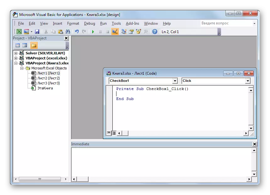
Execution of scenarios using ActiveX elements is possible using VBA tools, that is, by writing macros. Of course, it is much more complicated than using conditional formatting tools. The study of this issue is a separate big topic. Writing macros to specific tasks can only users with knowledge of programming and knowledge of work skills in Excel are much higher than the average level.

To go to the VBA editor, with which you can write a macro, you need to click on the item, in our case by checkbox, the left mouse button. After that, the editor window will be launched, in which you can write the code of the task being performed.

Lesson: How to create a macro in Excel

As you can see, there are several ways to install a tick in Excel. Which of the ways to choose, first of all depends on the installation objectives. If you want to just mark some object, it makes no sense to perform a task through the developer menu, as it will take a lot of time. It is much easier to use the insertion of a symbol or at all just dial the English letter "V" on the keyboard instead of a tick. If you want to organize specific scripts using a check mark, then in this case this purpose can only be achieved using the developer tools.