Extrapolation in Excel

There are cases when it is required to know the results of calculating the function outside the known area. This issue is especially relevant for the forecasting procedure. There are several ways to have several ways with which this operation can be performed. Let's look at them on specific examples.

Using extrapolation

In contrast to the interpolation, the task of which is the function of the function between two known arguments, extrapolation implies the search for solutions outside the known area. That is why this method is so in demand for forecasting.

Excel can use extrapolation, both for table values ​​and graphs.

Method 1: Extrapolation for tabular data

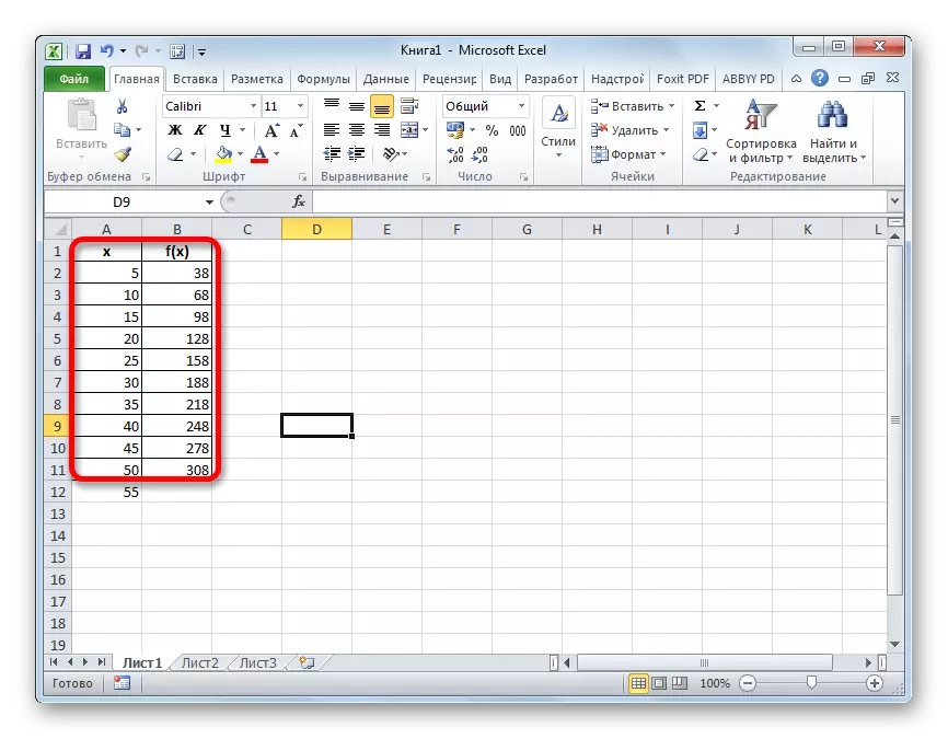
First of all, the extrapolation method to the contents of the table range is applicable. For example, take a table in which there are a number of arguments (x) from 5 to 50 and a number of corresponding function values ​​(F (X)). We need to find the value of the function for the argument 55, which is behind the limit of the specified data array. For these purposes, use the predicted function.

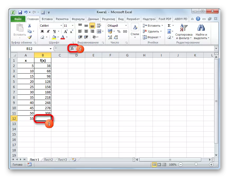
1. Select the cell in which the result of the calculations performed will be displayed. Click on the "Insert function" icon, which is posted at the formula string.



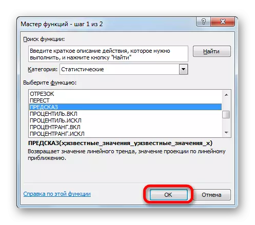
2. The functions wizard window starts. We carry out the transition to the category "Statistical" or "Full Alphabetical List". In the list that opens, we produce the search for the name "Predecz". Having found it, allocate, and then click on the "OK" button at the bottom of the window.



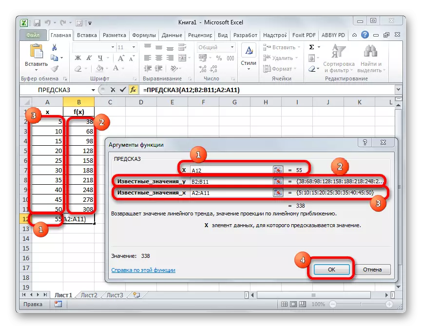
3. We move to the window of the arguments of the above function. It has only three arguments and the corresponding number of fields for their introduction.

   In the "X" field, specify the value of the argument, the function of which we should calculate. You can simply drive the desired number from the keyboard, and you can specify the coordinates of the cell if the argument is recorded on the sheet. The second option is even preferable. If we make an introduction in this way, in order to view the value of the function for another argument, we do not have to change the formula, but it will be enough to change the introductory in the corresponding cell. In order to specify the coordinates of this cell, if it was still selected the second option, it is enough to install the cursor to the appropriate field and select this cell. Her address will immediately appear in the argument window.

   In the "Known R values" field, you should specify the entire range of function ranges. It is displayed in the column "F (X)". Therefore, we set the cursor to the appropriate field and allocate the entire column without its name.

   In the "Known Values ​​X" field, you should specify all the values ​​of the argument that the function of the function corresponds to the above. These data are in the "X" column. In the same way as in the previous time, we allocate the column you need, after setting the cursor in the window of the argument window.

   After all the data is made, click on the "OK" button.



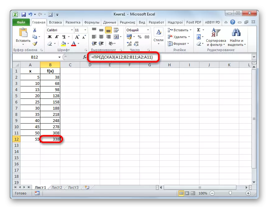
4. After these actions, the calculation result by extrapolation will be displayed in the cell, which was highlighted in the first paragraph of this instruction before starting the wizard of the functions. In this case, the function for the argument 55 is 338.



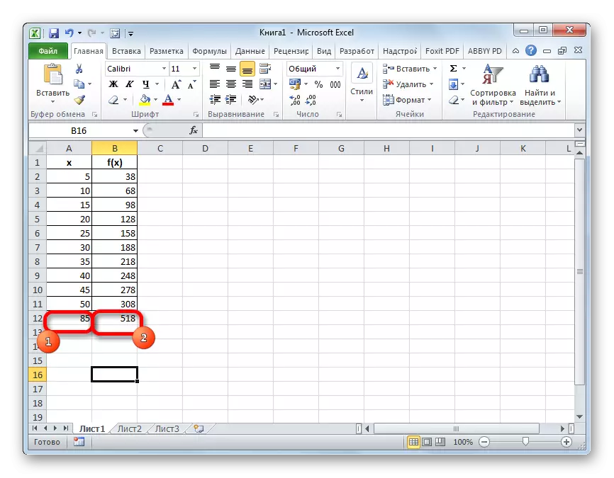
5. If after all the option was selected with the addition of a link to the cell, which contains the desired argument, then we can easily change it and view the function value for any other number. For example, the desired value for the argument 85 will be 518.

Lesson: Wizard Functions in Excel

Method 2: Extrapolation for schedule

Perform an extrapolation procedure for the graph by constructing a trend line.

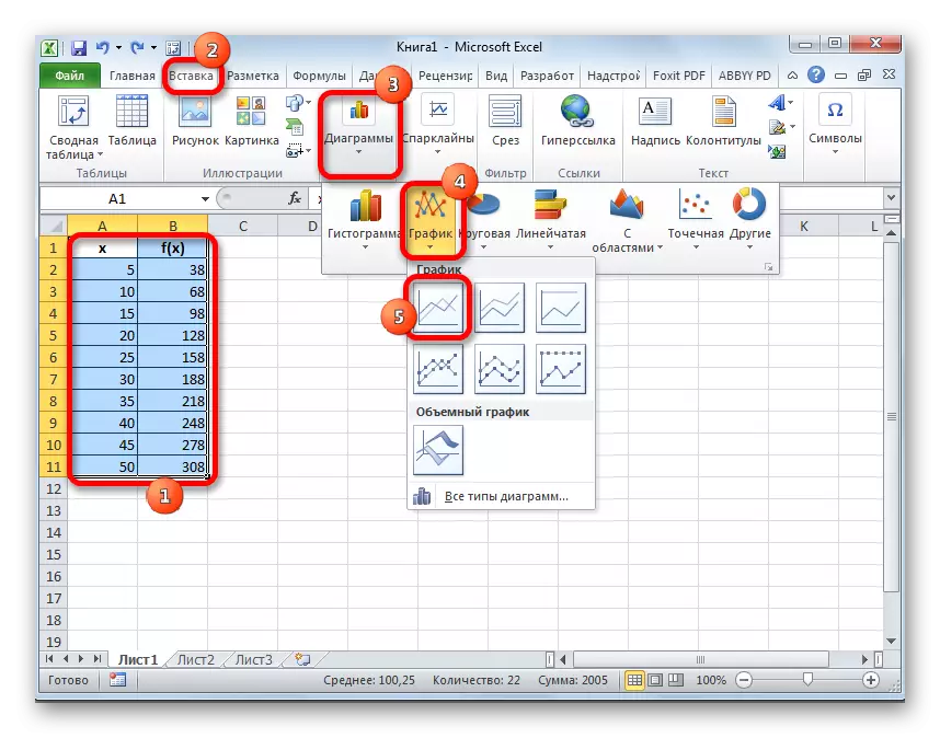
1. First of all, we build a schedule yourself. For this, the cursor with the left mouse button is highlighted by the entire area of ​​the table, including the arguments and the corresponding function values. Then, moving into the "Insert" tab, click on the "schedule" button. This icon is located in the "Chart" block on the tape ribbon. A list of available schedules appears. We choose the most suitable on their discretion.



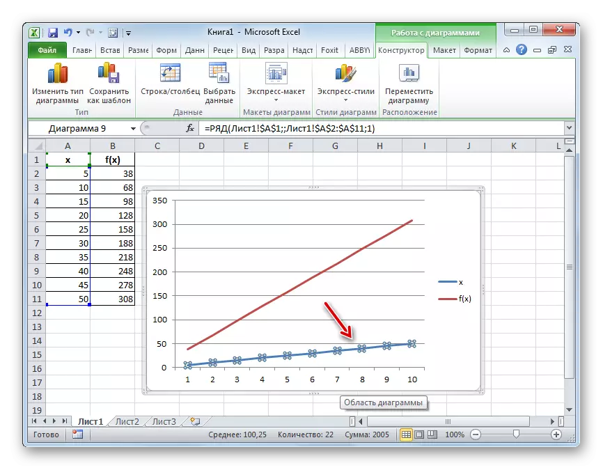
2. After the schedule is built, remove an additional argument line from it, highlighting it and pressing the Delete button on the computer keyboard.



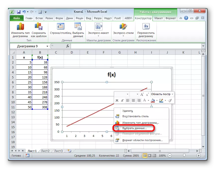
3. Next, we need to change the divisions of the horizontal scale, as it displays the not the values ​​of the arguments, as we need. To do this, click on the right mouse button on the diagram and in the list that appears, you stop at the "Select Data" values.



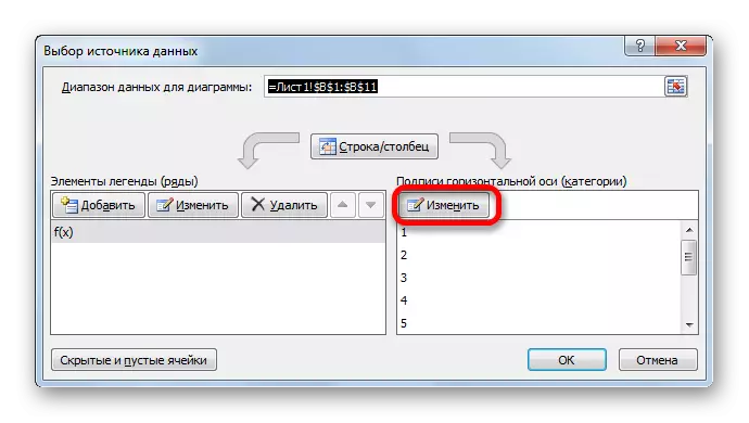
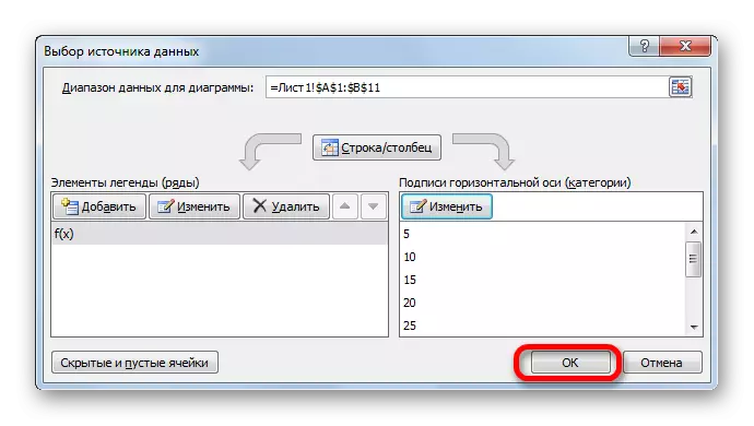
4. In the starting window of the data source selection window, click on the "Edit" button in the horizontal axis signature editing unit.



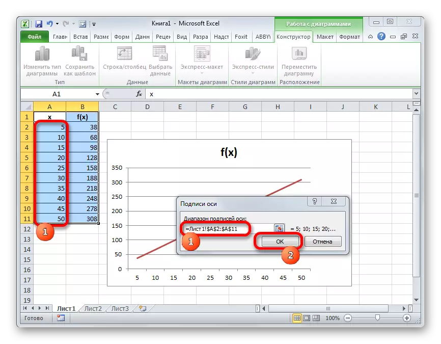
5. The axis signature installation window opens. We put the cursor in the field of this window, and then select all the data of the "X" column without its name. Then click on the "OK" button.



6. After returning to the data source selection window, we repeat the same procedure, that is, we click on the "OK" button.



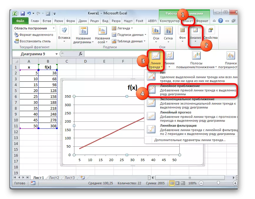
7. Now our schedule is prepared and can be directly proceeding to the construction of the trend line. Click on schedule, after which an additional set of tabs is activated on the tape - "work with charts". We move to the tab "Layout" and click on the "Trend Line" button in the "Analysis" block. Click on the "Linear approximation" or "Exponential approximation".



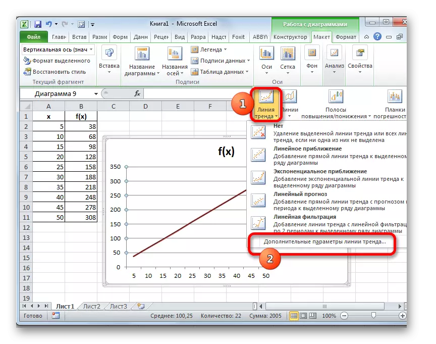
8. The trend line is added, but it is completely under the line of the graph itself, since we did not indicate the value of the argument to which it should strive. To do this again sequentially click on the "Trend Line" button, but now select the "Advanced Trend Line Parameters" item.



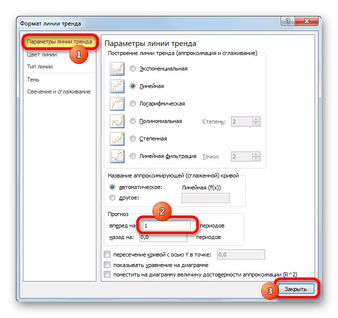
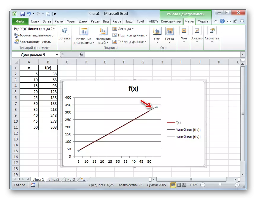
9. The trend line format window is started. In the "Trend Line Settings" section there is a "Forecast" settings block. As in the previous way, let's take an argument 55 for extrapolation. As you can see, it is for now the graph has a length to argument 50 inclusive. It turns out, we will need to extend it for another 5 units. On the horizontal axis it can be seen that 5 units are equal to one division. So this one period. In the "forward to" field, enter the value "1". Click on the "Close" button in the lower right corner of the window.



10. As we can see, the schedule was extended to the specified length using the trend line.

Lesson: How to build a trend line in Excel

So, we reviewed the simplest examples of extrapolation for tables and for graphs. In the first case, the predicted function is used, and in the second - the trend line. But on the basis of these examples, much more complex forecasting tasks can be solved.