Method 1: Pressing the line of hidden rows
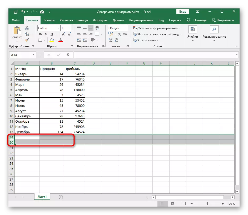
Although lines are not displayed in the table, they can be noticed on the left pane, where the numbers listed these lines are shown. The hidden range has a small rectangle, which should be shifted twice to display all the lines in it.
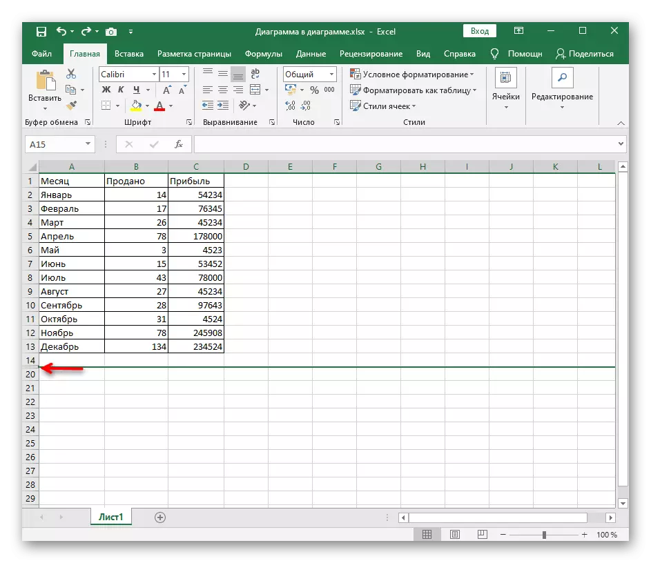
They will immediately stand out, and if the contents inside you can watch it. If such a method is not suitable due to the fact that the strings are scattered along a table or pressing simply not triggered, use other methods.
Method 2: Context Menu
This option will suit to those users who have hidden lines are consistently, but at the same time the click on them does not help or use the previous option is simply inconvenient. Then try making the fields visible through the context menu.
- Highlight the entire table or only those strings in the range of which are hidden.
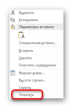
- Click any of the figures of the rows with the right mouse button and in the context menu that appears, select "Show".
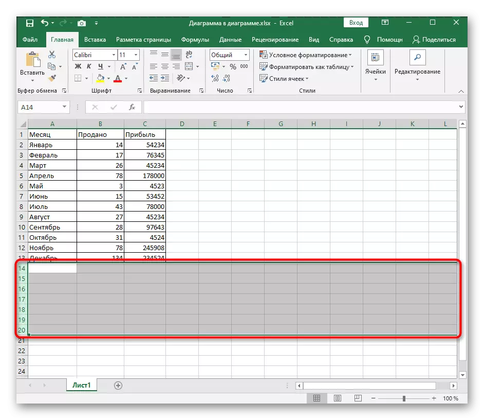
- The previously hidden lines will be immediately displayed in the table, which means that the task is successfully completed.
Method 3: Keyboard Keyboard
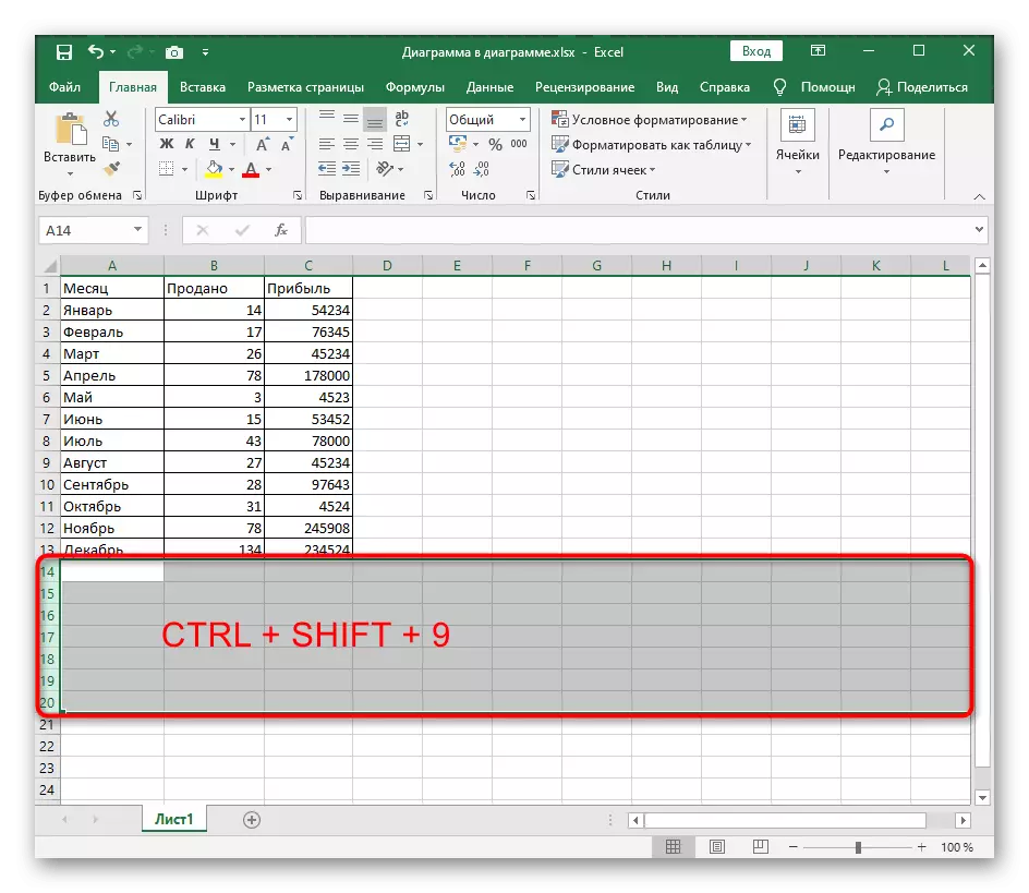
Another quick way to show hidden strings is to use the standard CTRL + SHIFT + 9 key combination, which is available in Excel by default. To do this, you do not need to search for the location of the fields or allocate the rows next to them. Just clamp this combination and immediately see the result.
Method 4: Menu "Format cells"
Sometimes to display all the rows immediately the optimal option becomes the use of a function in one of the Excel menu.
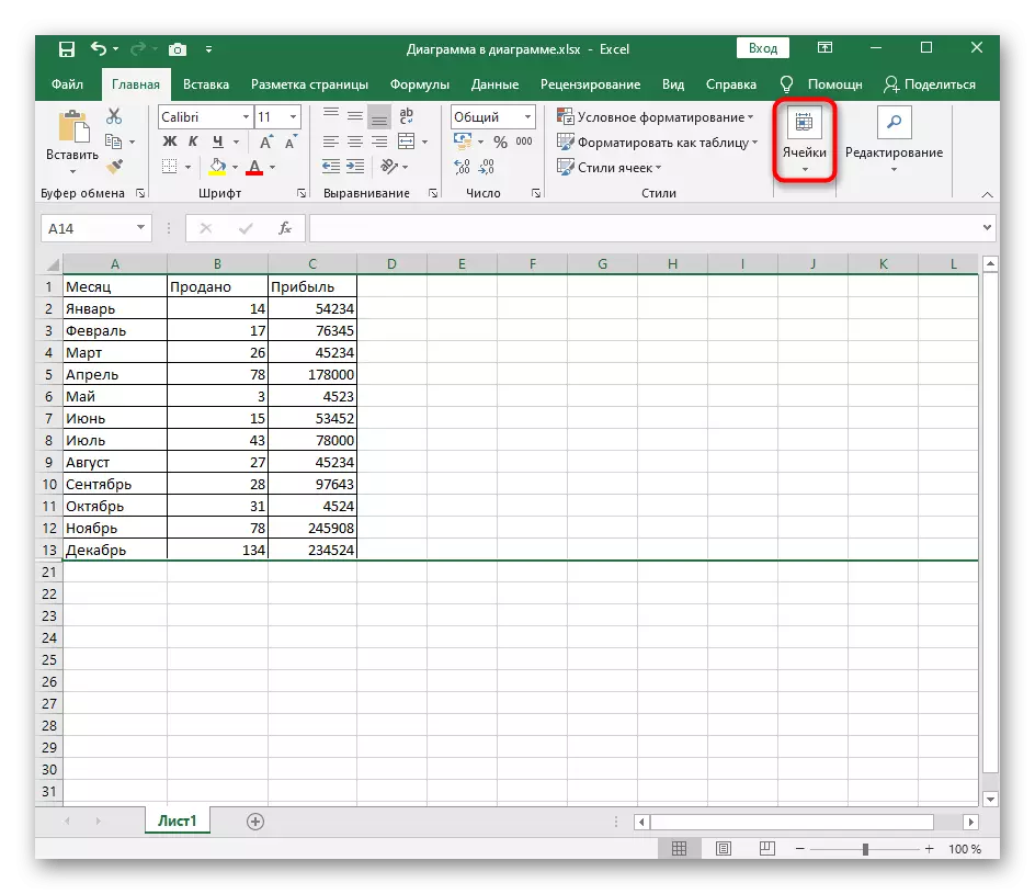
- Being on the Home tab, open the "Cell" block.
- Expand the "Format" drop-down menu.
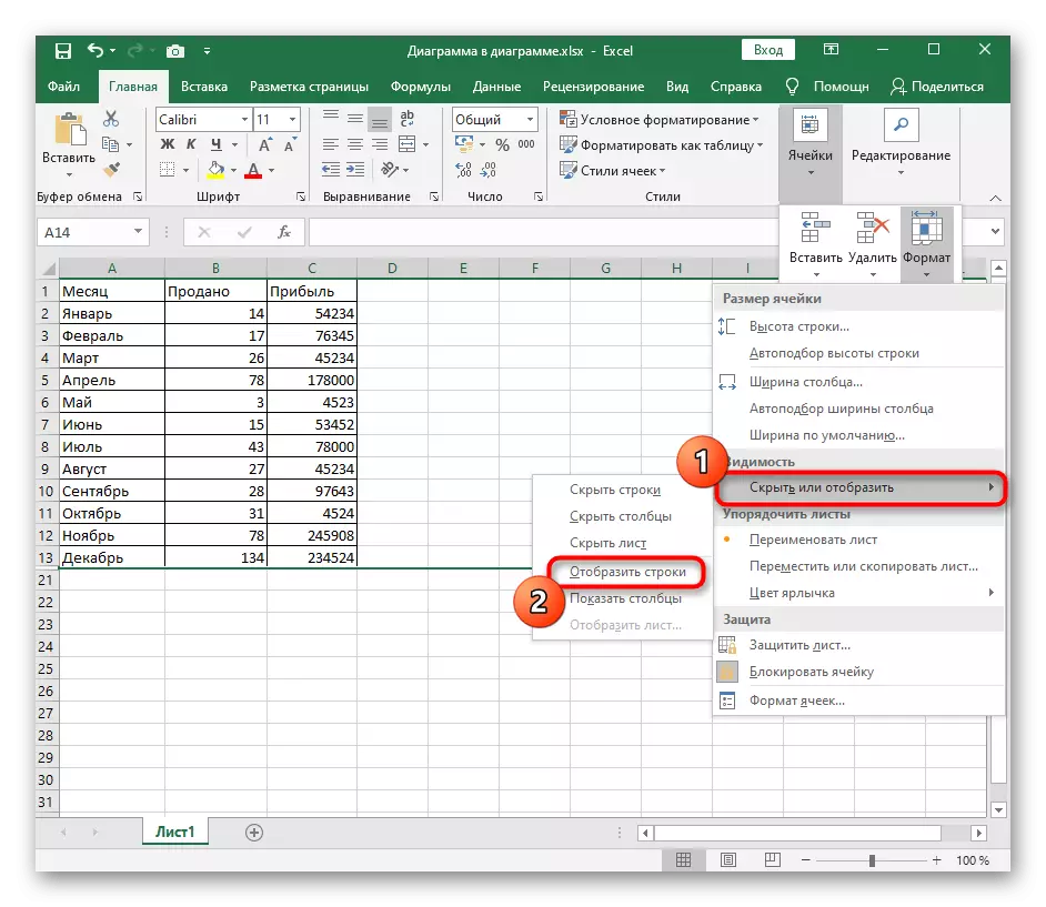
- In it, Mouse over to "Hide or Display" the cursor, where to select Rows.
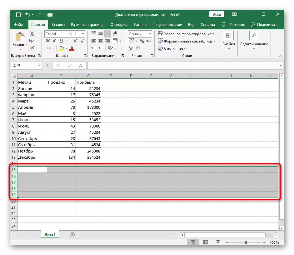
- The appears of the lines will be highlighted, so they will not be difficult to find them on the entire table. At the same time, the main thing is not to click on an empty place to accidentally do not remove the selection when searching.