Excel dispersion calculation

Among the many indicators that are used in statistics, it is necessary to select dispersion calculation. It should be noted that manually execution of this calculation is a rather tedious occupation. Fortunately, the Excel application has functions that allow you to automate the calculation procedure. We find out the algorithm for working with these tools.

Calculation of dispersion

Dispersion is an indicator of variation, which is the average square of deviations from the mathematical expectation. Thus, it expresses the scatter of numbers relative to the average value. The dispersion calculation can be carried out both by the general population and sample.

Method 1: Calculation by the General Agriculture

To calculate this indicator in Excel, the general set applies the function of the display. The syntax of this expression has the following form:

= D.g (number1; number2; ...)

A total of 1 to 255 arguments can be applied. As arguments they can act as numerical values ​​and references to the cells in which they are contained.

Let's see how to calculate this value for the range with numeric data.

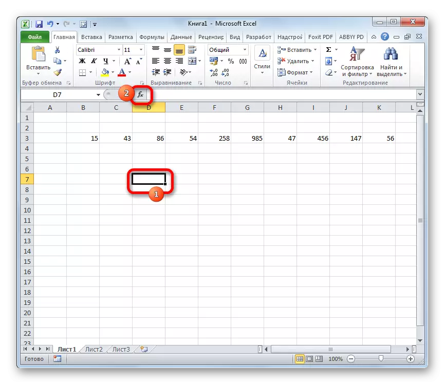
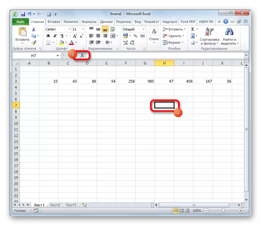
1. We produce the selection of the cell on the sheet into which the results of the dispersion calculation will be displayed. Click on the "Insert function" button, placed on the left of the formula string.



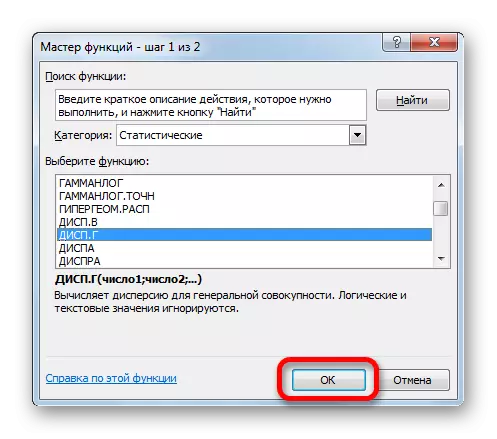
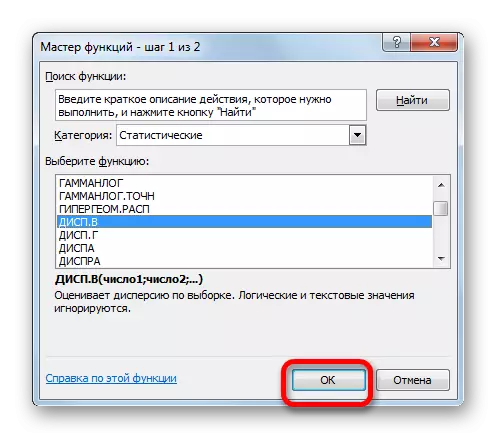
2. The functions master starts. In the "Statistical" category or "Full Alphabetical List", we perform a search for an argument with the name "LEG". After found, we allocate it and click on the "OK" button.



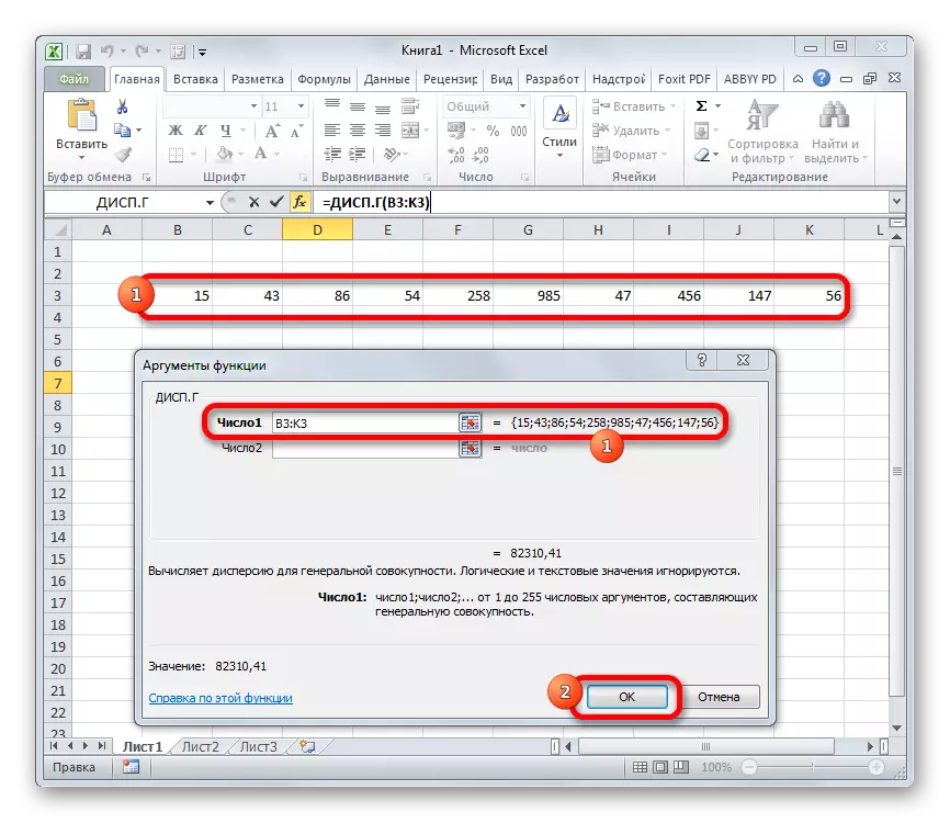
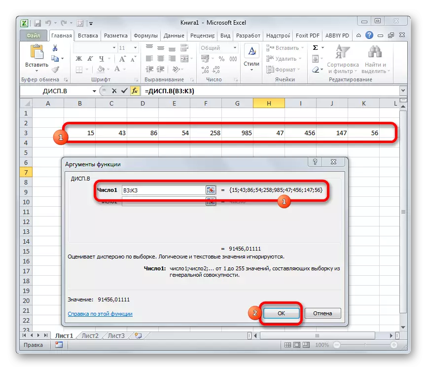
3. The display of the display of the display of the function is running. Install the cursor in the "Number1" field. We allocate the range of cells on the sheet, which contains a numeric row. If there are several such ranges, then you can also use the coordinates in the "Number2", "number3" field arguments window, etc. After all the data is made, click on the "OK" button.



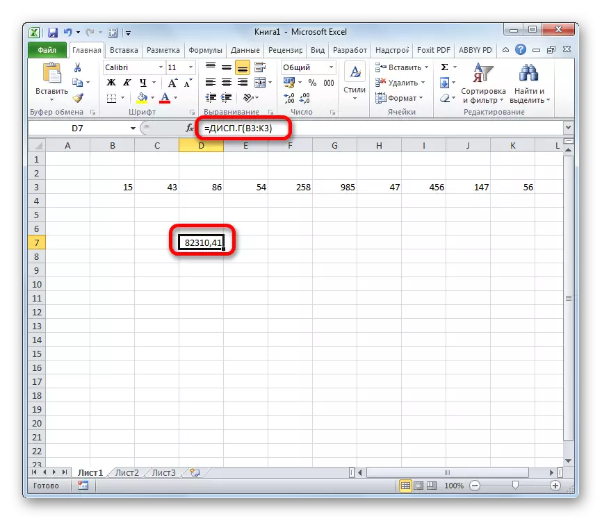
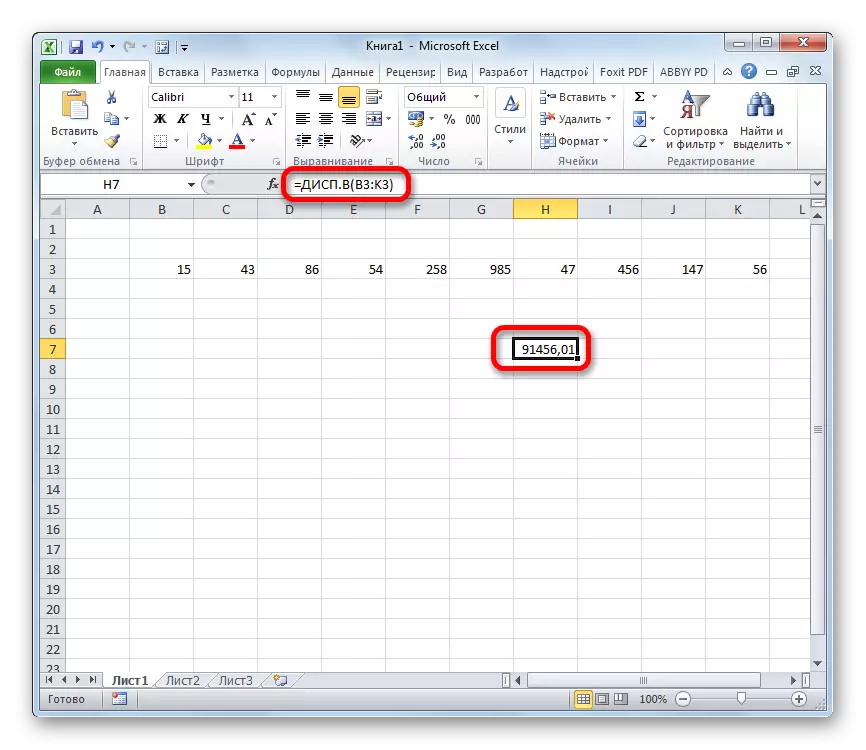
4. As you can see, after these actions calculated. The result of calculating the size of the variance by the general set is displayed in the pre-specified cell. This is exactly the cell in which the formula of the branch is directly located.

Lesson: Master of Functions in Excel

Method 2: sample calculation

In contrast to the calculation of the value according to the general set, in the calculation of the sample in the denominator, not a total number of numbers, but one less. This is done in order to correct the error. Excel takes into account this nuance in a special function, which is intended for this type of calculation - Dis.V. Its syntax is represented by the following formula:

= D (number1; number2; ...)

The number of arguments, as in the previous function, can also fluctuate from 1 to 255.

1. We highlight the cell and in the same way as the previous time, we launch the functions of the functions.



2. In the category "Full Alphabetical List" or "Statistical" looking for the name "Dis.V.". After the formula is found, we allocate it and make the click on the "OK" button.



3. The function of the function arguments is launched. Next, we do a fully in a similar way, as when using the previous operator: we set the cursor in the "number1" argument field and select the area containing the numerical row on the sheet. Then click on the "OK" button.



4. The result of the calculation will be removed in a separate cell.

Lesson: Other statistical functions in Excel

As you can see, the Excel program is able to significantly facilitate the calculation of the dispersion. This statistical value can be calculated by the application, both by the general population and sample. In this case, all user actions are actually reduced only to the indication of the range of the processed numbers, and the main work of Excel does itself. Of course, it will save a significant amount of user time.