How to make a sample in Excel: 4 working fashion

When working with Excel tables, it is often necessary to carry out the selection on a specific criterion or in several conditions. The program can do this in various ways using a series of tools. Let's find out how to make a sample in Excele using a variety of options.

Sampling

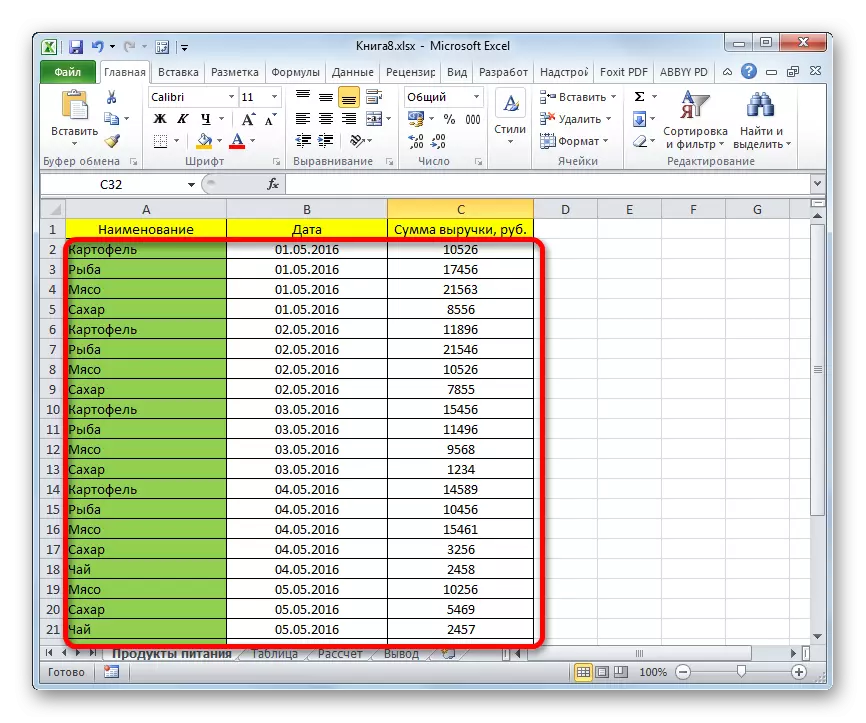
The data sample consists in the selection procedure from the total array of those results that satisfy the specified conditions, followed by the output of them on a sheet of a separate list or in the source range.

Method 1: Apply an extended autofilt

The easiest way to make the selection is the use of an extended autofilter. Consider how to do this on a specific example.

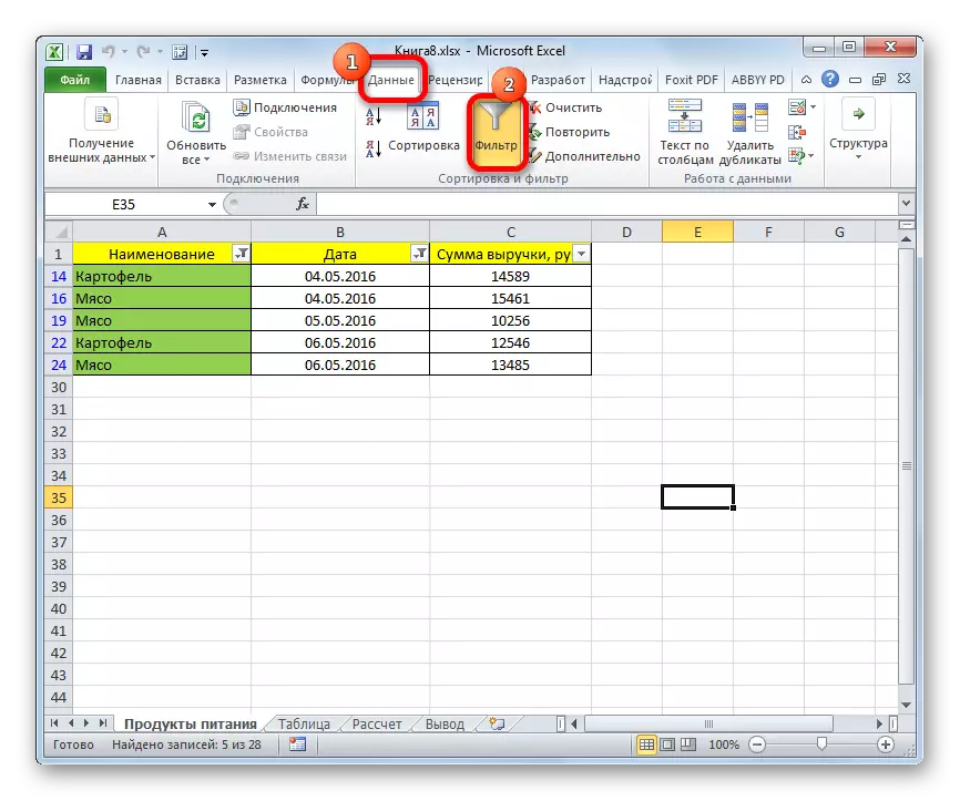
Select the area on the sheet, among the data of which you want to make a sample. In the Home tab, click on the "Sort and Filter" button. It is placed in the Editing Settings block. In the list that opens after this list, click on the "Filter" button.

There is an opportunity to do and differently. To do this, after selecting the area on the Sheet, we move to the "Data" tab. Click on the "Filter" button, which is placed on the tape in the Sort and Filter group.

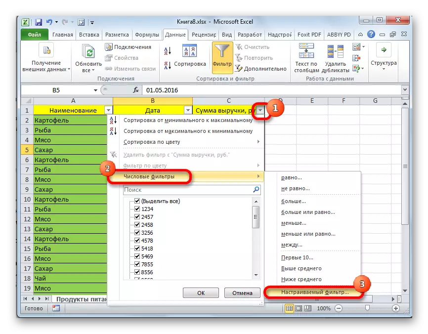
Enabling the filter through the Data tab in Microsoft Excel

After this action in the table header, pictograms appear to start filtering in the form of the edges of small triangles in the right edge of the cells. Click on this icon in the title of that column, according to which we wish to make a sample. In the menu running menu, go through the "Text Filters" item. Next, select the position "Customizable filter ...".

Switch to a custom filter in Microsoft Excel

The user filtering window is activated. In it, you can set a limit on which the selection will be made. In the drop-down list for a column of the numerical format cell, which we use for example, you can choose one of five types of conditions:
- equals;
- not equal;
- more;
- more or equal;
- smaller.
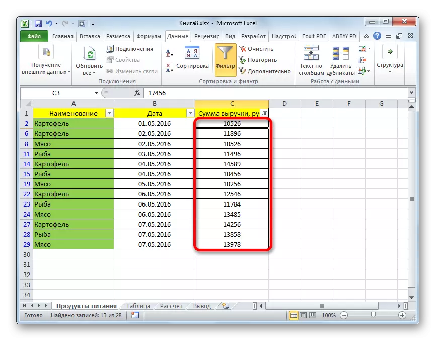
Let's set the condition as an example so as to select only the values for which the amount of revenue exceeds 10,000 rubles. We establish a switch to the "More" position. In the right field fit the value "10,000". To perform the action, click on the "OK" button.

As we see, after filtration, only lines remained, in which the amount of revenue exceeds 10,000 rubles.

But in the same column we can add the second condition. To do this, come back to the Custom Filtration window. As we can see, in its lower part there is another switch condition and the corresponding field for input. Let us now install the upper selection border of 15,000 rubles. To do this, set the switch to the "less" position, and in the field on the right fit the value "15000".
In addition, there is still a switch of conditions. He has two provisions "and" and "or". By default, it is installed in the first position. This means that only lines will remain in the sample that satisfy both restrictions. If it is set to "or" position, then the values that are suitable for any of the two conditions will remain. In our case, you need to set the switch to the "and" position, that is, leave this default setting. After all the values are entered, click on the OK button.

Installing the upper border in the user filter in Microsoft Excel

Now only lines remained in the table, in which the amount of revenue is not less than 10,000 rubles, but does not exceed 15,000 rubles.

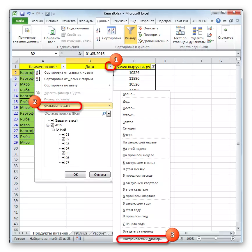
Filtration results at the bottom and upper border in Microsoft Excel

Similarly, you can configure filters in other columns. It is possible to maintain the filtering and on previous conditions that were set in the columns. So, let's see how the selection is taken using the filter for the dates format. Click on the filtration icon in the corresponding column. Consistently by clicking on the "Filter by date" list and the filter.

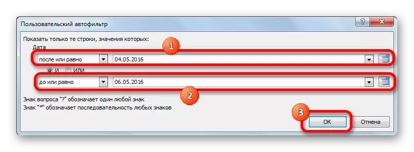
Switch to filtering by date in Microsoft Excel

The Custom Autofilt Run window starts again. Perform the selection of results in the table from 4 to 6 May 2016 inclusive. In the selection switch, as you can see, even more options than for a numerical format. Select the position "after or equal". In the field on the right, set the value "04.05.2016". In the bottom block, we set the switch to the "up to or equal" position. In the right field, enter the value "06.05.2016". Condition Compatibility Switch Leave in the default position - "and". In order to apply filtering in action, press the "OK" button.

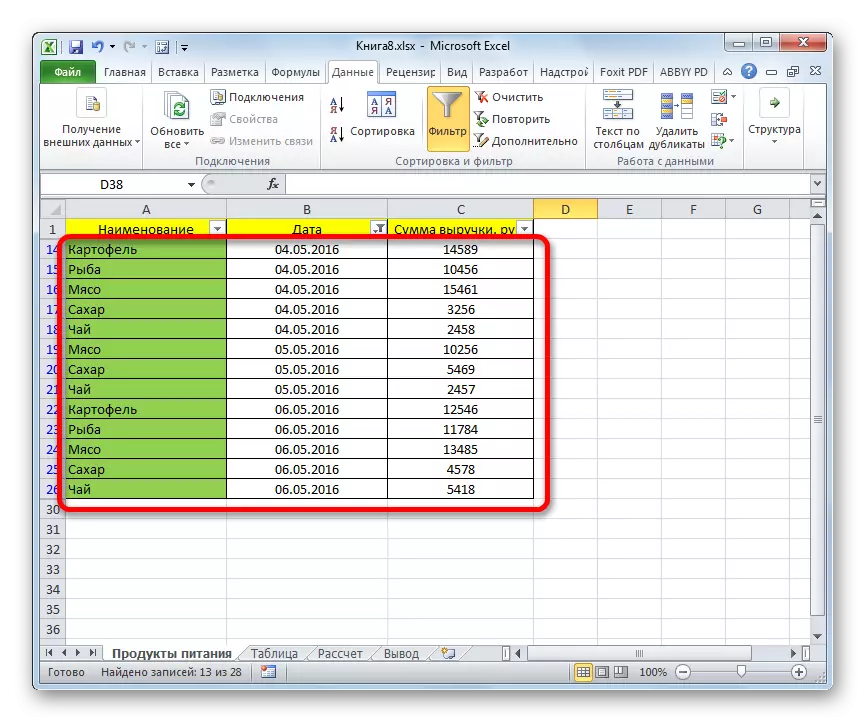
Users Filter for Date Format in Microsoft Excel

As you can see, our list has declined even more. Now only lines are left in it, in which the amount of revenue varies from 10,000 to 15,000 rubles for the period from 04.05 to 06.05.2016 inclusive.

Filtering results for sum and date in Microsoft Excel

We can reset filtering in one of the columns. Let's do it for revenue values. Click on the autofilter icon in the corresponding column. In the drop-down list, click on "Delete Filter" item.

Removing a filter from one of the columns in Microsoft Excel

As you can see, after these actions, the sample by the amount of revenues will be disabled, but will only take the selection by date (from 04/05/2016 to 06.05.2016).

Restrictions only by date in Microsoft Excel

This table has another column - "Name". It contains data in text format. Let's see how to form a sample using filtering through these values.
Click on the filter icon in the name of the column. Consistently go to the names of the List "Text Filters" and "Customizable Filter ...".

Transition to text filtering in Microsoft Excel

The user autofilter window opens again. Let's make a sample by the names of "Potatoes" and "Meat". In the first block, the Conditions switch set to the position "equal". In the field to the right of it fit the word "potatoes". The switch of the lower unit will also put the "equal" position. In the field opposite it, I make a record - "Meat". And now we carry out what they had not previously did: set the compatibility switch to the position "or". Now the line containing any of the specified conditions will be displayed on the screen. Click on the "OK" button.

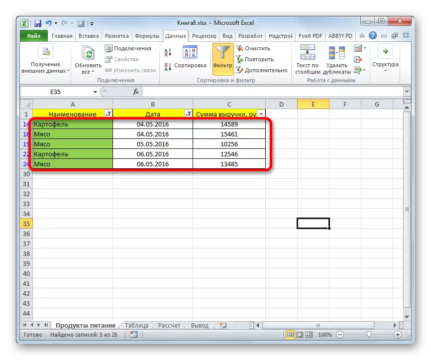
Filter for text format in Microsoft Excel

As you can see, there are restrictions on the date in the new sample (from 04.05.2016 to 06.05.2016) and by name (potatoes and meat). There are no restrictions on the amount of revenue.

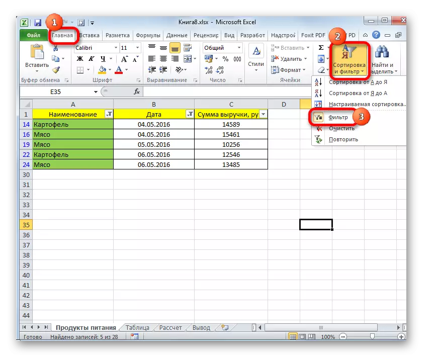
Date and name limitations in Microsoft Excel

You can completely remove the filter by the same methods that were used to install it. And it does not matter what method was used. To reset the filtering, while in the "Data" tab, click on the "Filter" button, which is located in the "Sort and Filter" group.

The second option involves the transition to the "Home" tab. We perform a click on the ribbon on the "Sort and Filter" button in the Editing unit. In the activated list, click on the "Filter" button.

Cleaning the filter in the Home tab in Microsoft Excel

When using any of the two above methods, filtering will be deleted, and the sample results are cleaned. That is, the table will be shown the entire array of the data that it has.

Lesson: Auto Filter Function in Excel

Method 2: Application of the array formula

Make the selection can also apply the complex formula of the array. In contrast to the previous version, this method provides for the output of the result in a separate table.

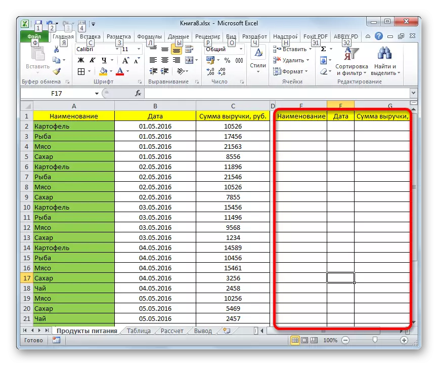
On the same sheet, we create an empty table with the same names of columns in the header as the source.

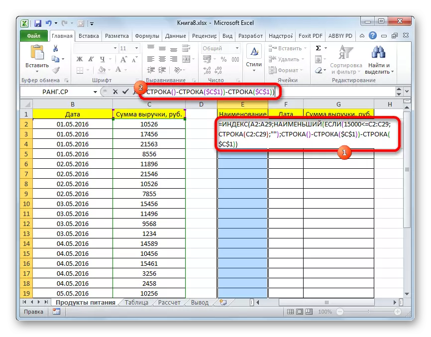
Creating an empty table in Microsoft Excel

Allocate all empty cells of the first column of the new table. Install the cursor in the formula string. Just here will be entered by a formula that produces a sample on the specified criteria. We will select the line, the amount of revenue in which exceeds 15,000 rubles. In our particular example, the introduced formula will look as follows:
= Index (A2: A29; smallest (if (15000
Naturally, in each particular case, the address of the cells and ranges will be yours. On this example, you can compare the formula with the coordinates on the illustration and adapt it for your needs.

Since this is an array formula, in order to apply it in action, you need to press the ENTER button, but the Ctrl + SHIFT + ENTER key combination. We do it.

The formula of the array is introduced into the name column in Microsoft Excel

Having highlight the second column with dates and installing the cursor in the formula string, we introduce the following expression:
= Index (B2: B29; smallest (if (15000
Click the CTRL + SHIFT + ENTER key combination.

The formula of the array is introduced into the dates column in Microsoft Excel

Similarly, in a column with revenue, enter the formula of the following content:
= Index (C2: C29; smallest (if (15000
Again, type the CTRL + SHIFT + ENTER key combination.
In all three cases, only the first value of the coordinates is changing, and the rest of the formula is completely identical.

The array formula is entered in the revenue column in Microsoft Excel

As we see, the table is filled with data, but its appearance is not entirely attractive, moreover, the values of the dates are filled in it incorrectly. It is necessary to correct these shortcomings. The incorrectness of the date is related to the fact that the format of the cells of the corresponding column is common, and we need to set the date format. We highlight the entire column, including cells with errors, and click on highlighting the right mouse button. In the list that appears, go through the "Cell Format ...".

Transition to cell formatting in Microsoft Excel

In the formatting window that opens, open the "Number" tab. In the "Numeric formats" block allocate the "date" value. On the right side of the window, you can select the desired date display type. After the settings are exhibited, click on the "OK" button.

Now the date is displayed correctly. But, as we see, the entire bottom of the table is filled with cells that contain the erroneous value "# number!". In essence, these are those cells, data from the sample for which they did not have enough. It would be more attractive if they were displayed at all empty. For these purposes, we use conditional formatting. We highlight all table cells, except for the header. While in the Home tab, click on the "Conditional Formatting" button, which is in the "Styles" tool block. In the list that appears, select the "Create Rule ..." item.

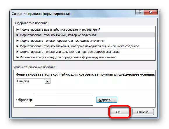
Transition to the creation of the rule in Microsoft Excel

In the window that opens, select the type of rule "format only cells that contain". In the first field, under the inscription "Format only the cells for which the following condition," select the "error" position. Next, click on the "Format ..." button.

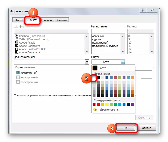
Switch to the selection of format in Microsoft Excel

In the formatting window running, go to the "Font" tab and select white in the appropriate field. After these actions, click on the "OK" button.

On the button with exactly the same name, click after returning to the Creating Conduct Window.

Creating a formatting condition in Microsoft Excel

Now we have a finished sample on the specified limit in a separate properly decorated table.

Lesson: Conditional formatting in Excel

Method 3: Sampling on several conditions using the formula

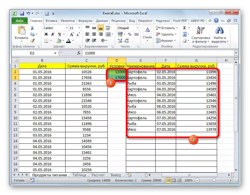
Just as when using the filter, using the formula you can select on several conditions. For example, take the same source table, as well as an empty table, where results will be output, with already performed numerical and conditional formatting. We will establish the first limitation of the lower border of the selection by revenue in 15,000 rubles, and the second condition of the upper border of 20,000 rubles.

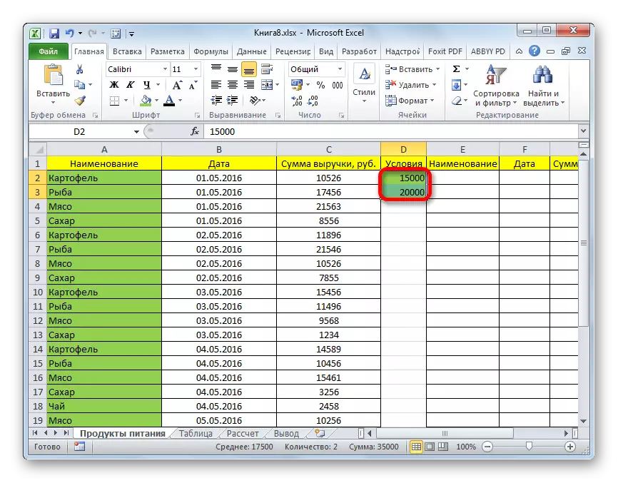
Enter in a separate column, boundary conditions for sampling.

As in the previous method, alternately allocate the empty columns of the new table and enter the corresponding three formulas in them. In the first column we introduce the following expression:
= Index (A2: A29; smallest (if (($ D $ 2 = C2: C29); line (C2: C29); ""); string (C2: C29) -strkok ($ C $ 1)) - line ($ C $ 1))
In the subsequent columns, fit exactly the same formulas, only by changing the coordinates immediately after the name of the operator, the index to the corresponding columns we need, by analogy with the previous method.
Each time after entering, do not forget to gain the CTRL + SHIFT + ENTER key combination.

Result of the sample on several conditions in Microsoft Excel

The advantage of this method before the previous one is that if we want to change the boundaries of the sample, it will not be necessary to change the solid formula itself, which in itself is quite problematic. It is enough in the column of conditions on the sheet to change the boundary numbers on those that are needed by the user. The results of the selection will immediately automatically change.

Changing the sampling results in Microsoft Excel

Method 4: Random Sampling

In the exile, with the help of a special formula, it is also possible to apply random selection. It is required in some cases when working with a large amount of data when you need to present a common picture without a comprehensive analysis of all data of the array.

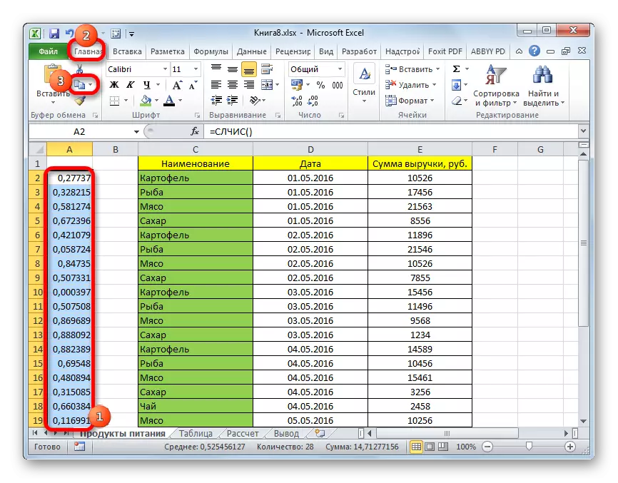
To the left of the table skip one column. In the cell of the next column, which is located opposite the first cell with the data of the table, enter the formula:
= Adhesive ()
This feature displays a random number. In order to activate it, click on the ENTER button.

In order to make a whole column of random numbers, set the cursor to the lower right corner of the cell, which already contains the formula. The filling marker appears. I stretch it down with the left mouse button parallel to the table with the data until its end.

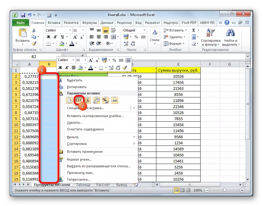
Now we have a range of cells filled with random numbers. But, he contains the Formula of Calc. We need to work with clean values. To do this, copy to an empty column on the right. Select the range of cells with random numbers. Located in the "Home" tab, click on the "Copy" icon on the ribbon.

We highlight an empty column and click right-click, calling the context menu. In the "Insert Parameters" toolbar, select the "Value" clause, depicted as pictograms with numbers.

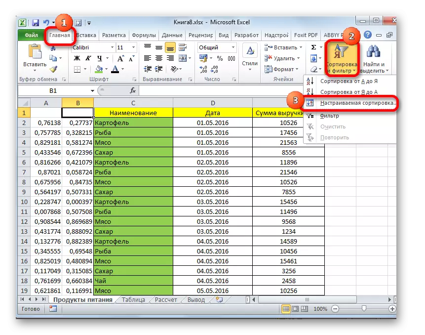
After that, while in the "Home" tab, click on the already familiar icon of the "Sort and Filter" icon. In the drop-down list, stop the selection at the "Custom Sorting" item.

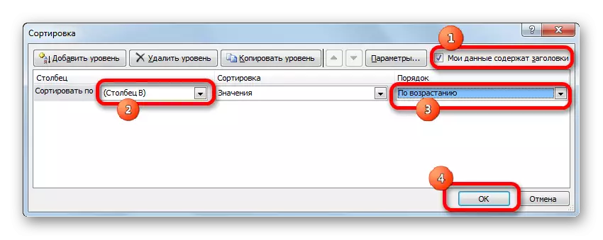
Transition to custom sorting in Microsoft Excel

The sorting settings window is activated. Be sure to install a tick opposite the parameter "My data contain headlines" if the cap is available, but no ticks. In the "Sort by" field, specify the name of that column in which the copied values of random numbers are contained. In the "Sort" field, leave the default settings. In the "order" field, you can choose the parameter as "ascending" and "descending". For a random sample, this value does not have. After the settings are manufactured, click on the "OK" button.

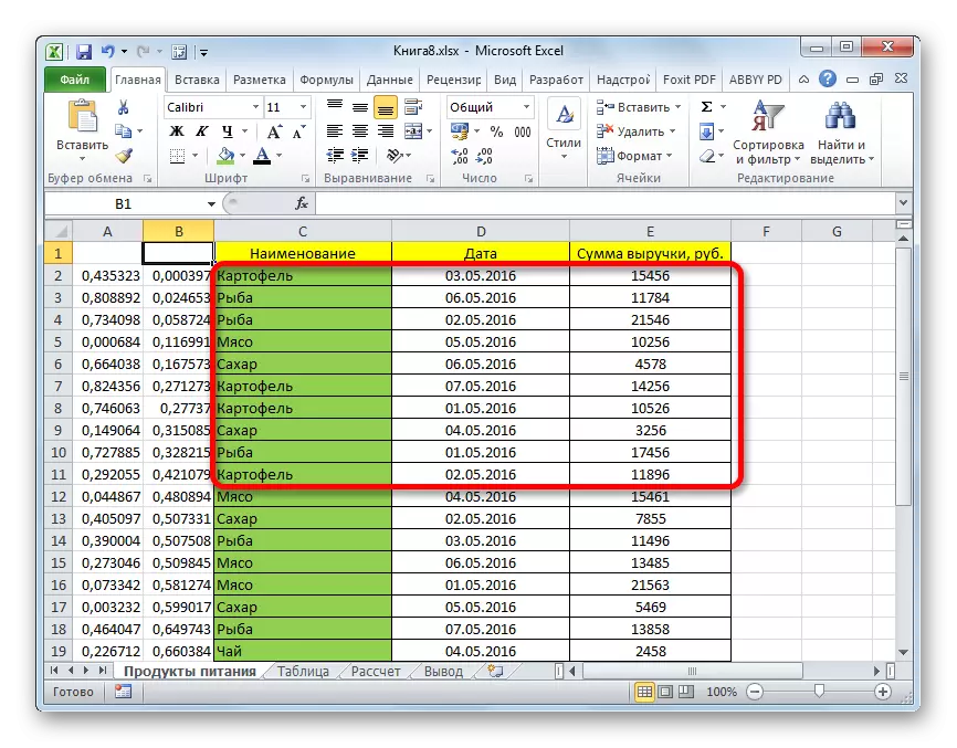
After that, all values of the table are built in ascending order or decrease of random numbers. You can take any number of the first lines from the table (5, 10, 12, 15, etc.) and they can be considered the result of a random sample.

Lesson: Sorting and filtering data to Excel

As you can see, the sample in the Excel table can be produced, both using autofilter and applying special formulas. In the first case, the result will be displayed in the source table, and in the second - in a separate area. It is possible to produce selection, both one condition and several. In addition, you can make a random sample using the adhesive function.