How to build a parabola in Excel

The construction of a parabola is one of the well-known mathematical operations. Quite often it applies not only for scientific purposes, but also in purely practical. Let's find out how to make this procedure using the Excel application toolkit.

Creation of parabola

Parabola is a graph of the quadratic function of the next type f (x) = ax ^ 2 + bx + c . One of the noteworthy properties is the fact that Parabola has a form of a symmetric figure consisting of a set of points equidistant from the director. By and large, the construction of the parabola in the Excel environment is not much different from building any other graph in this program.

Creating a table

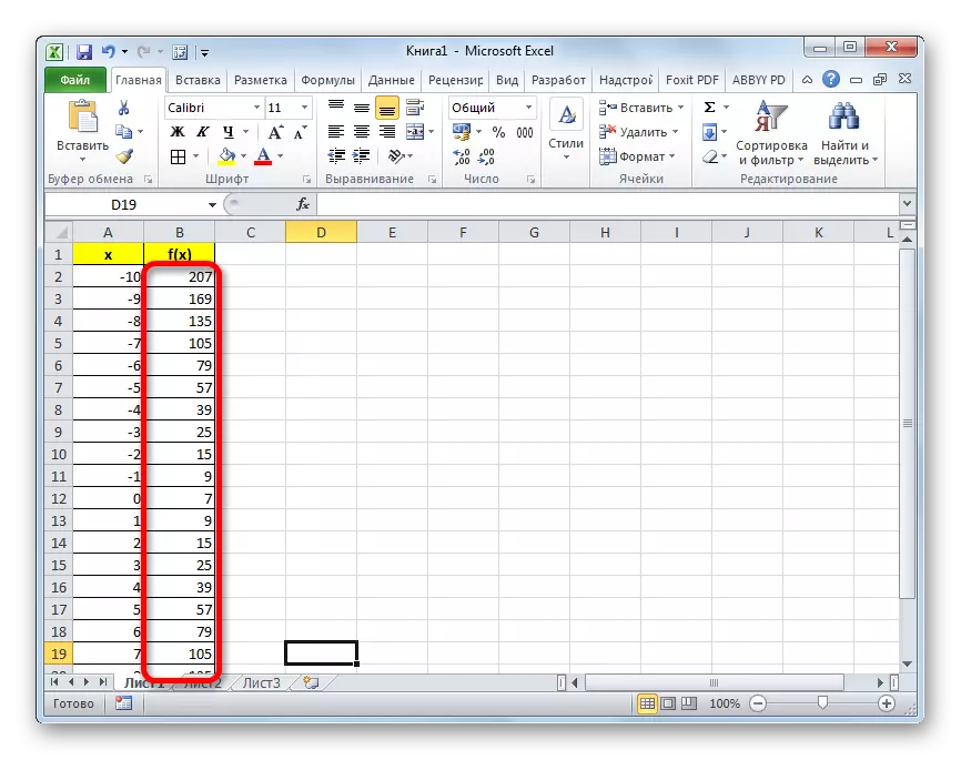
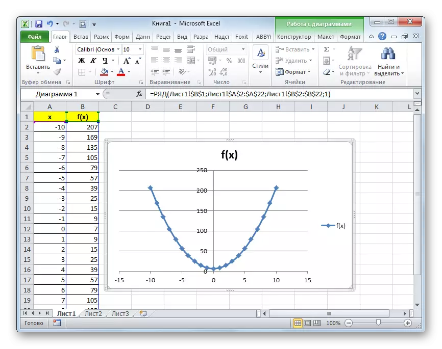
First of all, before proceeding to building a parabola, you should build a table on the basis of which it will be created. For example, take the graph of the function of the function f (x) = 2x ^ 2 + 7.

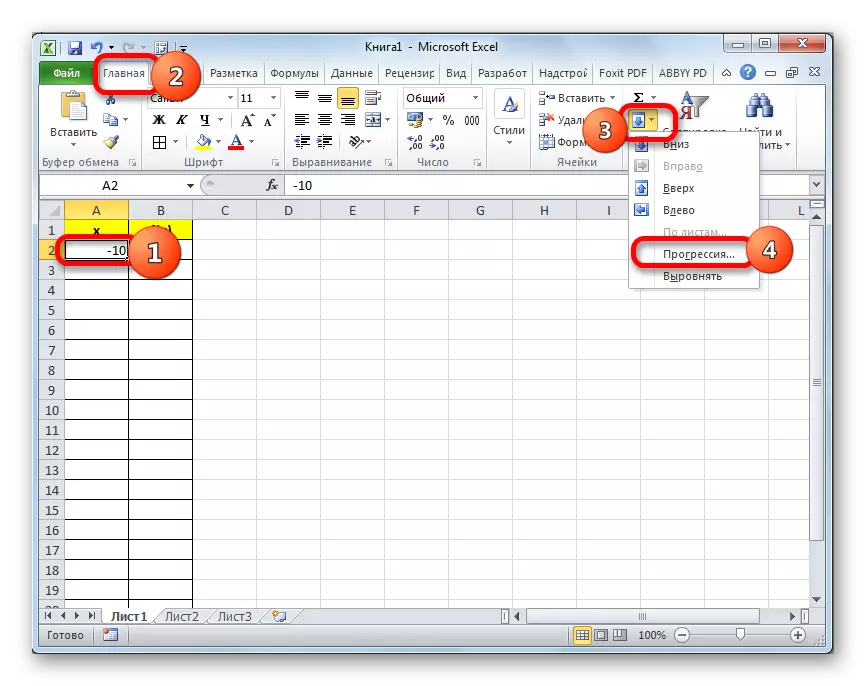
1. Fill out a table with x values ​​from -10 to 10 in step 1. This can be done manually, but easier for these purposes to use the progression instruments. To do this, in the first cell of the column "X" we enter the value "-10". Then, without removing the selection from this cell, go to the "Home" tab. We click on the "Progression" button, which is posted in the Editing group. In the activated list, choose the position "Progression ...".



2. Activation of the progression adjustment window is activated. In the "Location" block, the button should be rearranged to the position "on columns", since the series "X" is placed in the column, although in other cases it may be necessary to set the switch to the "on lines" position. In the "Type" block, leave the switch in the arithmetic position.

   In the "Step" field, we enter the number "1". In the "Limit value" field, indicate the number "10", as we consider the X range from -10 to 10 inclusive. Then click on the "OK" button.



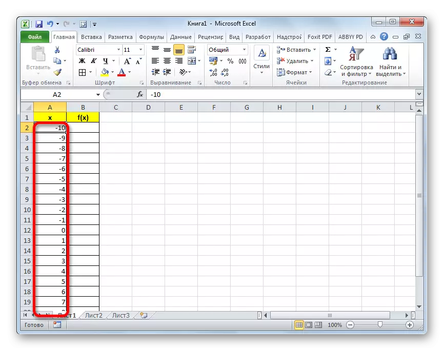
3. After this action, the entire column "X" will be filled with the data we need, namely, the numbers in the range from -10 to 10 in increments of 1.



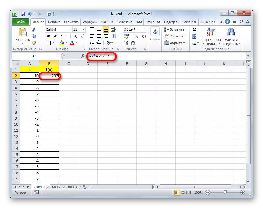
4. Now we will have to fill in the column "F (X)". To do this, based on the equation (F (x) = 2x ^ 2 + 7), we need to enter an expression on the next model of this column to the following layout:

   = 2 * x ^ 2 + 7

   Only instead of the value of x we ​​substitute the address of the first cell of the column "X", which we just filled out. Therefore, in our case, the expression will take the form:

   = 2 * A2 ^ 2 + 7



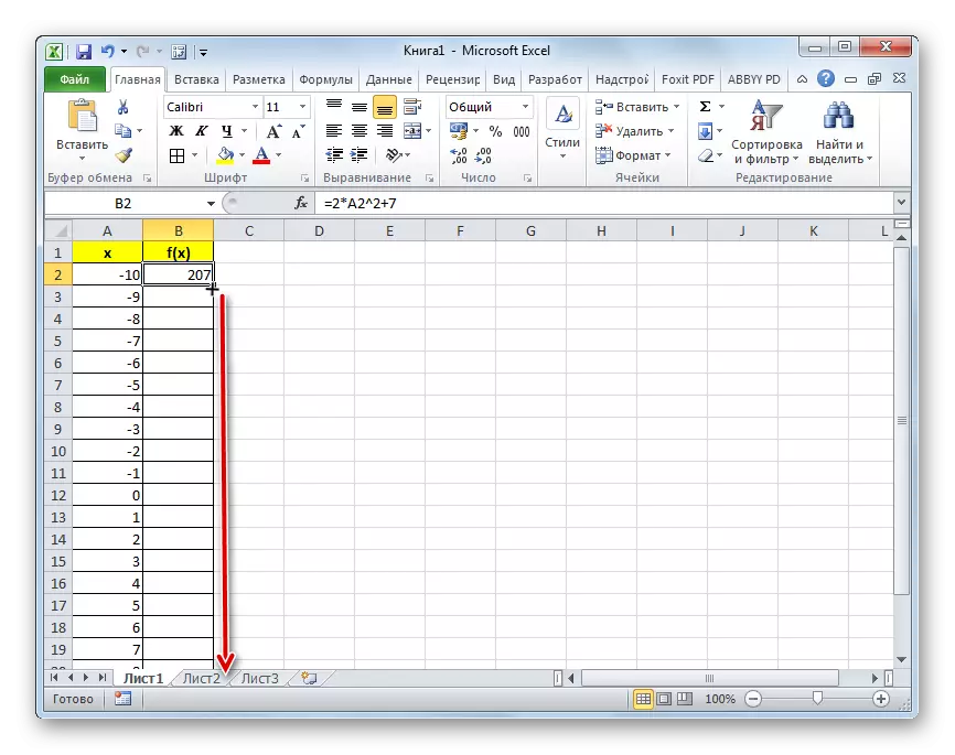
5. Now we need to copy the formula and for the entire lower range of this column. Given the basic properties of Excel, when copying all X values ​​will be delivered to the corresponding column cells "F (X)" automatically. To do this, we put the cursor to the lower right corner of the cell, in which the formula has already been placed, recorded by us a little earlier. The cursor should be converted to a filling marker, having a look of a small cross. After the conversion occurred, clamp the left mouse button and pull the cursor down to the end of the table, then let go of the button.



6. As you can see, after this action, the column "F (X)" will also be filled.

On this formation, the table can be considered completed and move directly to the construction of the schedule.

Lesson: How to make autocomplete in exile

Building graphics

As already mentioned above, now we have to build a schedule.

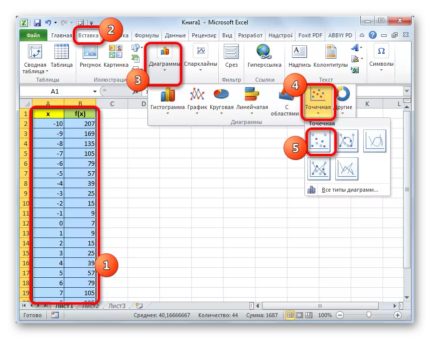
1. Select the table with the cursor by holding the left mouse button. Move into the "Insert" tab. On the tape in the "chart block" click on the "Spot" button, since it is this type of graph that is most suitable for the construction of a parabola. But that's not all. After clicking on the above button, a list of points of point diagrams opens. Choose a point diagram with markers.



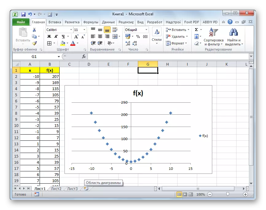
2. As we see, after these actions, Parabola is built.

Lesson: How to make a chart in exile

Editing chart

Now you can edit the resulting schedule.

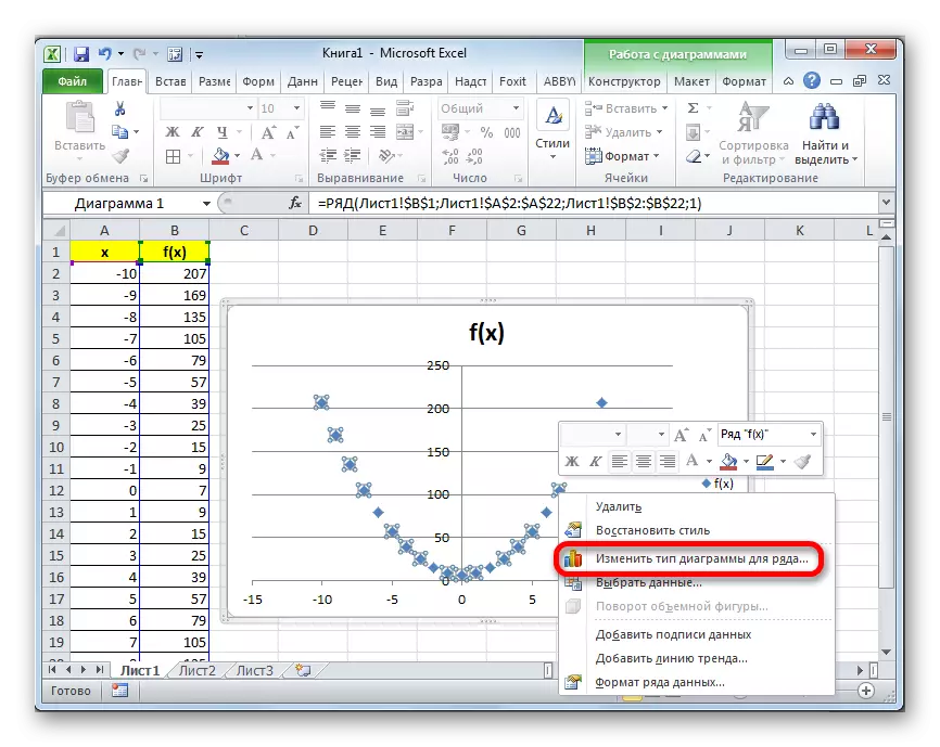
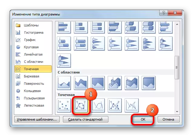
1. If you do not want Parabola to be displayed in the form of points, and there was a more familiar view of the line curve, which connects these points, click on any of them right-click. The context menu opens. In it you need to choose the item "Change the type of diagram for a row ...".



2. The window selection window opens. Select the name "Spot with smooth curves and markers." After the choice is made, click on the "OK" button.



3. Now the chart of parabola has a more familiar look.

In addition, you can make any other types of editing the received parabola, including the change in its name and names of the axes. These editing receivers do not go beyond the limits of action to work in Excel with diagrams of other species.

Lesson: How to sign the axis of the chart in Excel

As you can see, building a parabola into Excel is not fundamentally different from building another type of graph or chart in the same program. All actions are made based on a predetermined table. In addition, it is necessary to consider that the point type of chart is most suitable for building a parabola.