

The main functionality of Microsoft Excel is tied to formulas, thanks to which, with this tabular processor, you can not only create a table of any complexity and volume, but also calculate those or other values in its cells. Counting the amount in the column is one of the simplest tasks with which users face most often, and today we will tell about the various options for its solution.
We consider the amount in the column in Excel
Calculate the sum of one or another values in the EXCEL's columns, you can automatically, using the basic program tools. In addition, it is possible to normal viewing of the final value without writing it into the cell. Just from the last, the most simple we will begin.Method 1: View a total amount
If you just need to see the total value in the column, in the cells of which contain certain information, while constantly keeping this amount before your eyes and create a formula for its calculation, do the following:
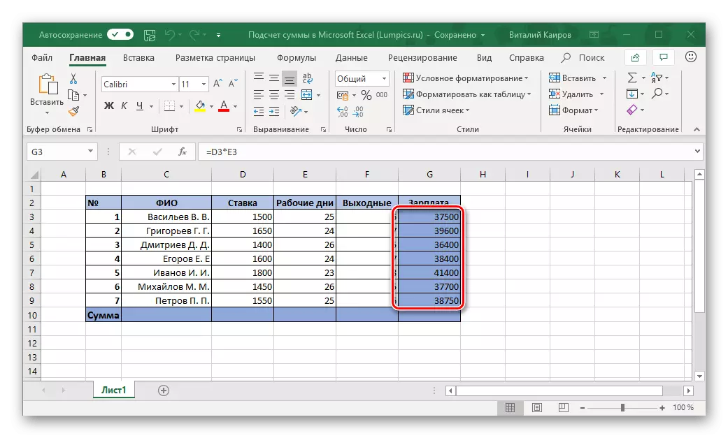
- Using the mouse, select the range of cells in the column, the amount of the values in which you want to count. In our example, it will be cells from 3 to 9 columns G.
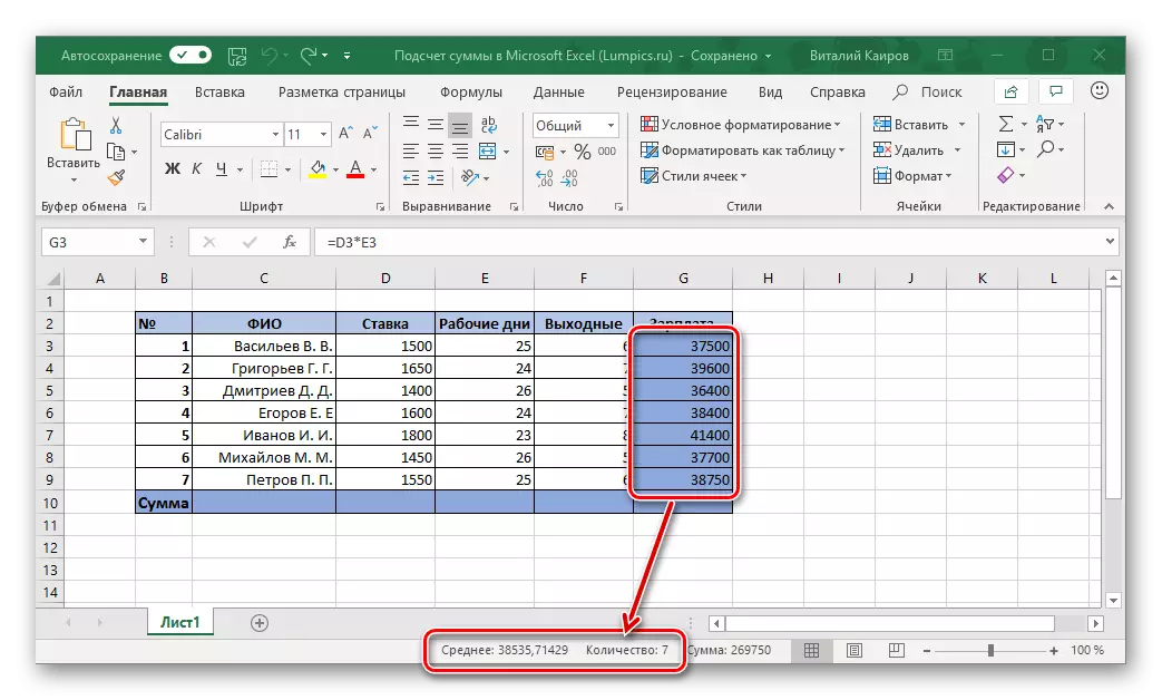
- Take a look at the status bar (the lower panel of the program) - the amount will be indicated there. This value will be displayed solely until the range of cells is highlighted.
- Additionally. Such a summation works, even if there are empty cells in the column.

Moreover, in a similar way, it is possible to calculate the amount of all values in the cells immediately from several columns - it is enough just to highlight the required range and look at the status bar. More on how it works, we will tell in the third method of this article, but already on the example of the template formula.


Note: To the left of the amount indicated the number of selected cells, as well as the average value for all numbers specified in them.
Method 2: Avosumn
Obviously, much more often the amount of values in the column is required to keep before your eyes, see it in a separate cell and, of course, track changes, if they are entered in the table. The optimal solution in this case will be automatic summation performed using a simple formula.
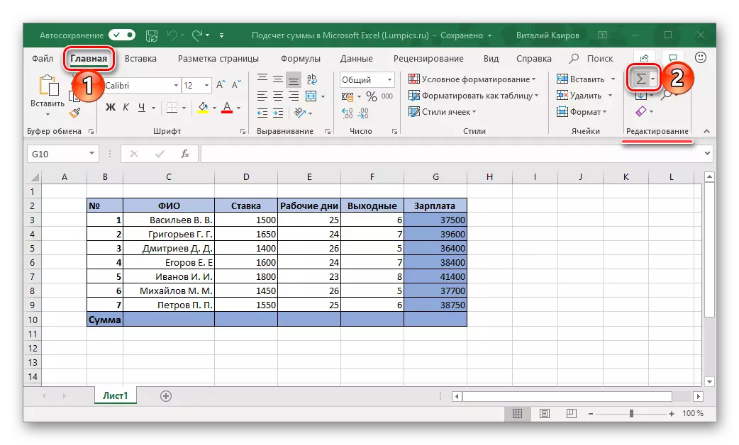
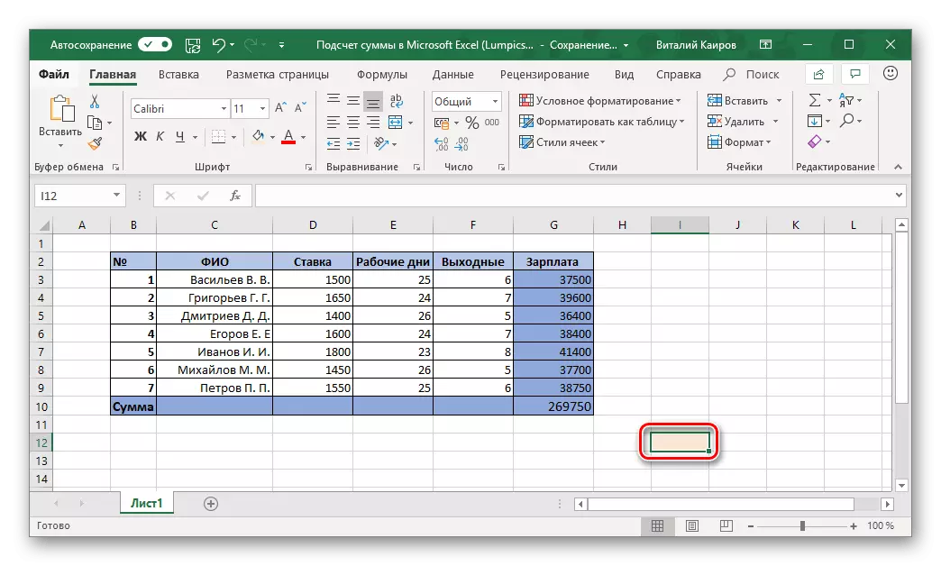
- Press the left mouse button (LKM) on an empty cell, located under the sum of which you want to count.
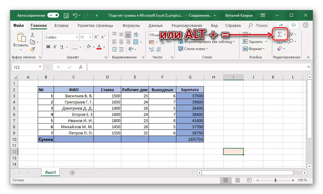
- Click the LKM on the "Amount" button located in the Editing toolbar (Main tab). Instead, you can use the key combination "Alt" + "=".
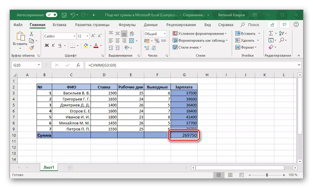
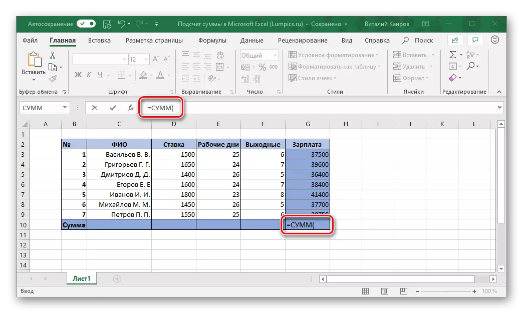
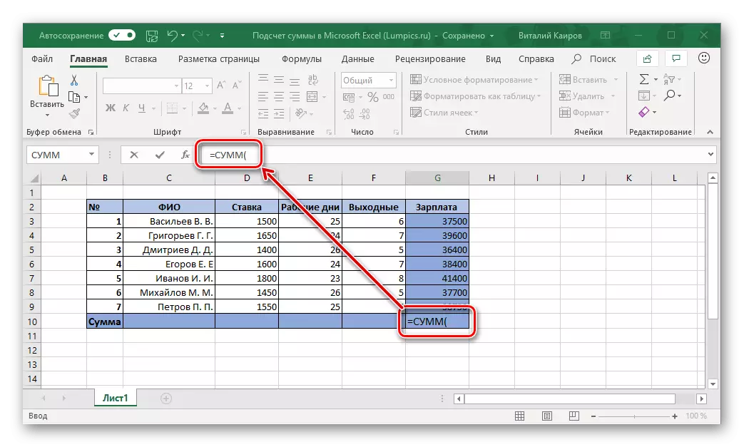
- Make sure that in the formula that appeared in the selected cell and the formula line, the address is the first and last of those that must be summarized and press "ENTER".

You will immediately see the sum of the numbers in the entire range.

Note: Any change in cells from the dedicated range will instantly reflect on the final formula, that is, the result in it will also change.
It happens that the amount should be removed not in that cell, which is under the summable, and in some other, possibly located completely in another column of the table. In this case, act as follows:
- Highlight the cell in which the sum of values will be calculated.
- Click on the "sum" button or use the hot keys to enter the same formula.
- Using the mouse, select the range of cells that you want to sum up and press "ENTER".

Advice: Select the range of cells and a little different way - click the LKM on the first of them, then clamp the key SHIFT And click on the latter.

Almost the same way can be summed up the values at once from several columns or individual cells, even if there will be empty cells in the band, but all this is more.
Method 3: Mall of Multiple Columns
It happens that it is necessary to calculate the amount not in one, but immediately in several columns of the spreadsheet of Excel. It is done almost the same as in the previous way, but with one small nuance.
- Click the LCM on the cell in which you plan to display the sum of all values.
- Click on the "Sum" button on the toolbar or use the key combination of keys intended for entering this formula.
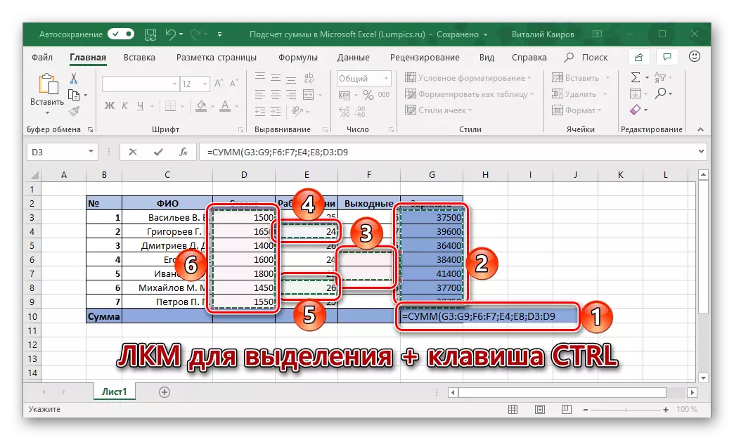
- The first column (above formula) will already be highlighted. Therefore, clamp the "Ctrl" key on the keyboard and select the following range of cells, which must also be included in the calculated amount.
- Further, in a similar way, if it is still necessary, by pressing the "CTRL" key, select the cells from other columns, the contents of which should also be included in the final amount.

Press "ENTER" to count, after which the resulting calculation will appear in the box intended for the formula and string on the toolbar.


Note: If the columns that need to count in a row, you can allocate them all together.

It is easy to guess that it is possible to calculate the amount of values in separate cells, consisting both in different columns and within one.
To do this, you just need to highlight the cell for the formula, click on the "sum" button or on the hot keys, select the first range of cells, and then by clicking the "Ctrl" key, allocate all other "plots" of the table. Having done this, just press "ENTER" to display the result.

As in the previous method, the amount formula can be recorded in any of the free table cells, and not only in the one that is under the summable.
Method 4: Summation manually
Like any formula in Microsoft Excel, the "amount" has its own syntax, and therefore it can be spelled out manually. Why do you need it? At least, so that in this way you can accurately avoid random errors in the allocation of the summable range and the indication of the cells included in it. Moreover, even if you make a mistake on some of the steps, it will be just as simple as a banal typo in the text, which means that you will not need to do all the work from scratch, as it sometimes has to do.
Among other things, the independent entry of the formula allows you to place it not only anywhere in the table, but also on any of the sheets of a particular electronic document. Is it worth saying that in this way not only the columns and / or their ranges can be summed up, but also simply individual cells or groups of those, excluding those that should not be taken into account?
The formula of the amount has the following syntax:
= Sums (summable cells or range such)
That is, everything that must be summarized is written in brackets. The values indicated inside the brackets should look like this:
- For range: A1: A10 - This is the sum of the 10 first cells in column A.
- For individual cells: A2; A5; A7; A10 - The sum of the cells No. 2, 5, 7.10 column A.
- Mixed value (ranges and separate cells): A1; A3: A5; A7; A9: 15 - The sum of the cells No. 1, 3-5, 7, 9-15. It is important to understand that there should be no additional separator symbol between the ranges and single cells.


And now we turn directly to the manual summation of the values in the Eksel spreadsheet column / columns.
- Highlight by pressing the LCM that cell that will contain a final formula.
- Enter the following in it:
= Sums (
After that, start alternately enter the formulamable ranges and / or individual cells in the line, not forgetting the separators (":" - for the range, ";" - for single cells, introduce without quotes), that is, do everything according to that algorithm, The essence of which we described in detail above.
- When specifying all the items that you want to sum up and making sure that you did not miss anything (you can navigate not only at the addresses in the formula row, but also backlit selected cells), close the bracket and press "ENTER" to count.

Note: If you have noticed an error in the final formula (for example, an excess cell has entered there, or some kind of missed), simply manually enter the correct designation (or delete too much) in the formula row. Similarly, if and when it is necessary, you can proceed with separator symbols in the form «;» and «:».

As you probably could have already guessed, instead of manually entering the addresses of cells and their ranges, you can simply select the necessary items using a mouse. The main thing is not to forget to hold the "Ctrl" key when you go from the allocation of one item to another.


Self, manual counting amounts in column / columns and / or individual table cells - the task is not the most convenient and fast in the implementation. But, as we have already told above, this approach provides much more wide opportunities for interacting with the values and allows you to instantly correct random errors. But whether it is completely manually by entering each variable from the keyboard in the formula, or to use the mouse and hotkeys to do it - solve only you.
Conclusion
Even such, it would seem, a simple task, as the counting of the amount in the column, is solved in the Microsoft Excel table processor at once in several ways, and each of them will find its use in one situation or another.