How to calculate interest in Excel

When working with tabular data, it is often necessary to calculate the percentage of the number or calculate the share as a percentage of the total amount. This feature provides Microsoft Excel. But unfortunately, not every user knows how to use tools to work with interest in this program. Let's find out how to calculate the percentage in Excel.

Excel interest calculation

Excel can perform many mathematical tasks, including the simplest calculation of interest. The user, depending on the needs, will not be difficult to calculate the percentage of the number and a number of percentage, including in tabular data options. To do this, you should only take advantage of certain formulas.

Option 1: Percentage calculation of the number

First of all, let's find out how to calculate the amount of the share as a percentage of one number from the other.

1. The calculation formula is as follows: = (number) / (general_sum) * 100%.
2. To demonstrate calculations in practice, we learn how much percent is the number 9 from 17. Select the cell where the result will be displayed and be sure to pay attention to which format is specified on the Home tab in the "Number" tab. If the format is different from the percentage, be sure to install the "Percentage" parameter in the field.
3. After that, write the following expression: = 9/15 * 100%.



4. However, since we set a percentage of cell format, add "* 100%" to add. It is enough to limit ourselves to the record "= 9/17".



5. To view the result, press the ENTER key. As a result, we get 52.94%.

Now take a look at how to calculate interest, working with tabular data in cells.

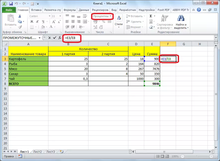
1. Suppose we need to count how much percent is the proportion of the specific type of product from the total amount specified in a separate cell. To do this, in a string with the name of the goods click on an empty cell and set the percentage format in it. We put the sign "=". Next, click on the cell, indicating the value of the implementation of a specific type of product "/". Then - by cell with a total amount of sales for all goods. Thus, in the cell for the output of the result, we recorded the formula.



2. To view the value of the calculations, click Enter.



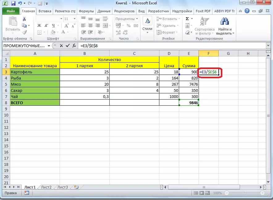
3. We found out the definition of interest in percent only for one line. Is it really necessary to introduce similar calculations for each next line? Not necessarily. We need to copy this formula to other cells. However, since the link to the cell with the total amount should be constant so that the displacement does not occur, then in the formula before the coordinates of its row and column, we put the "$" sign. After that, reference from relative turns into absolute.



4. We carry the cursor to the lower right corner of the cell, the value of which is already calculated, and by holding the mouse button, stretch it down to the cell, where the total amount is inclusive. As you can see, the formula is copied to all other cells of the table. Immediately visible the result of calculations.



5. You can calculate the percentage of individual components of the table, even if the total amount is not displayed in a separate cell. After formatting the cell to output the result in the percentage format, we put the "=" sign in it. Next, click on the cell, whose share must know, put the sign "/" and gain the amount from which the percentage is calculated. You don't need to turn the link to the absolute in this case.



6. Then click ENTER and by dragging with copying the formula into the cells, which are located below.

Option 2: The calculation of the percentage number

Now let's see how to calculate the number of the total amount percent from it.

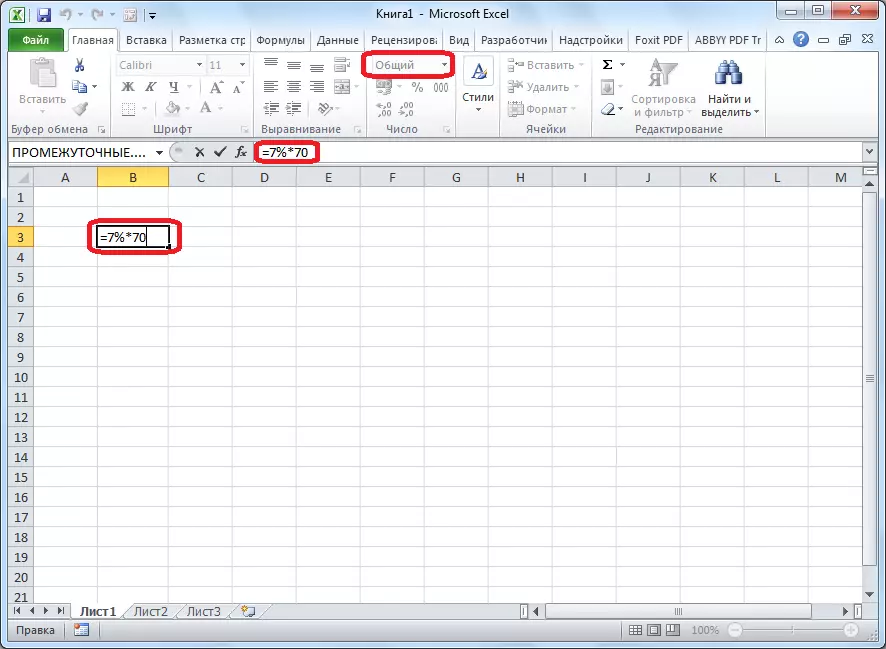
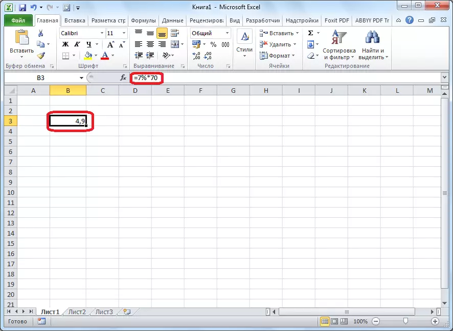
1. The formula for the calculation will have the following form: the value_procerant% * Total_sum. Consequently, if we need to calculate what number is, for example, 7% of 70, then simply enter the expression "= 7% * 70" into the cell. Since in the end we get a number, not a percentage, then in this case it is not necessary to set a percentage format. It must be either common or numeric.



2. To view the result, press ENTER.



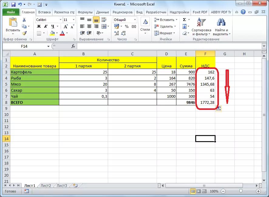
3. This model is quite convenient to apply to work with tables. For example, we need from revenue of each name of the goods to calculate the amount of VAT values, which is 18%. To do this, choose an empty cell in a row with the name of the goods. It will become one of the composite elements of the column in which the amount of VAT will be indicated. I format it into the percentage format and put the sign "=". We recruit the number 18% and the "*" sign on the keyboard. Next, click on the cell in which the amount of revenue from the sale of this product name is. Formula is ready. Change the format of cell percentage or make links absolute should not be.



4. To view the results of the calculation of the Enter.



5. Copy the formula into other cells dragging down. Table with data on the amount of VAT is ready.

As you can see, the program provides an opportunity to work comfortably with percentages. The user can calculate both a fraction of a certain number in percent and the number from the total percentage. Excel can be used to work with percentages as a regular calculator, but also with it easily and automate work to calculate interest in the tables.