How to build a trend line in Excel

One of the important components of any analysis is to determine the main trend of events. Having this data can be a forecast for the further development of the situation. This is especially clearly visible on the example of the trend line on the schedule. Let's find out how in the Microsoft Excel program you can build it.

Trend line in Excel

The Excel application provides the ability to build a trend line with a graph. At the same time, the initial data for its formation is taken from a pre-prepared table.

Building graphics

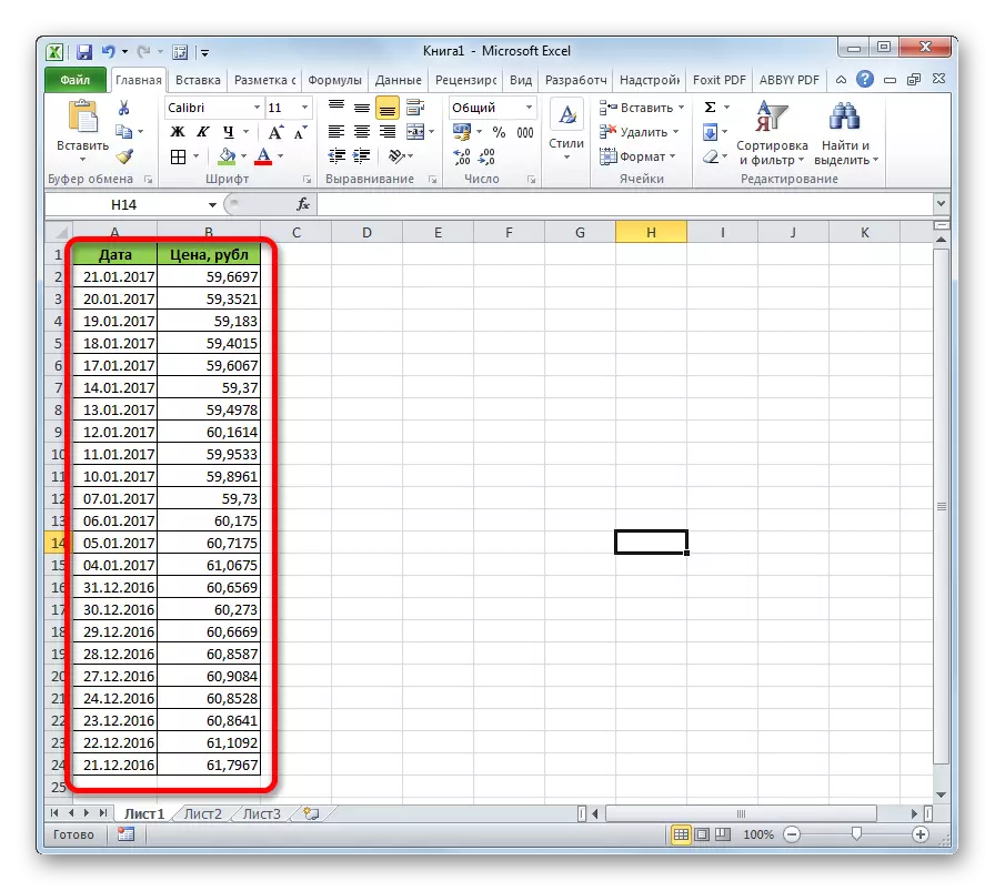
In order to build a chart, you need to have a ready-made table, on the basis of which it will be formed. As an example, we take data on the value of the dollar in rubles for a certain period of time.

1. We build a table where in one column will be temporary segments (in our case of dates), and in the other - the value, the dynamics of which will be displayed in the graph.



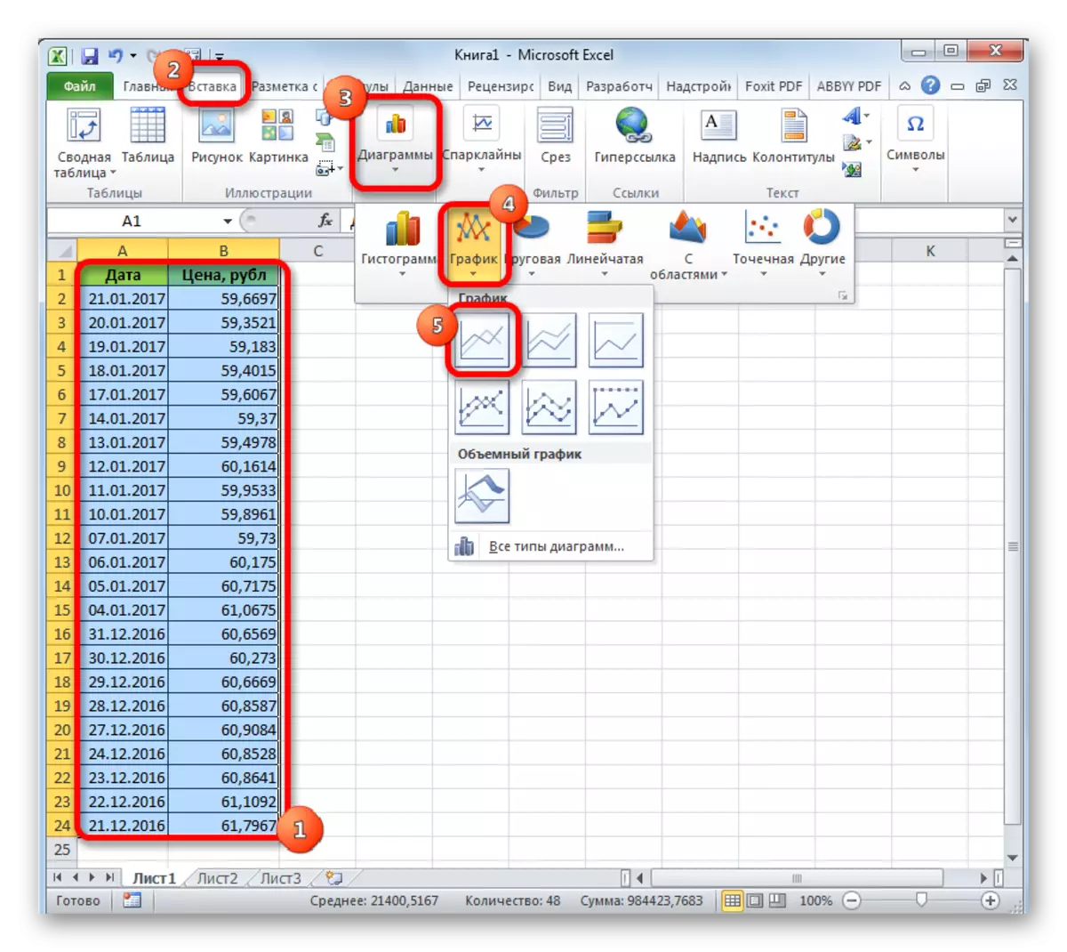
2. Select this table. Go to the "Insert" tab. There on the tape in the "diagram" tool block by clicking on the "Schedule" button. From the list presented, choose the very first option.



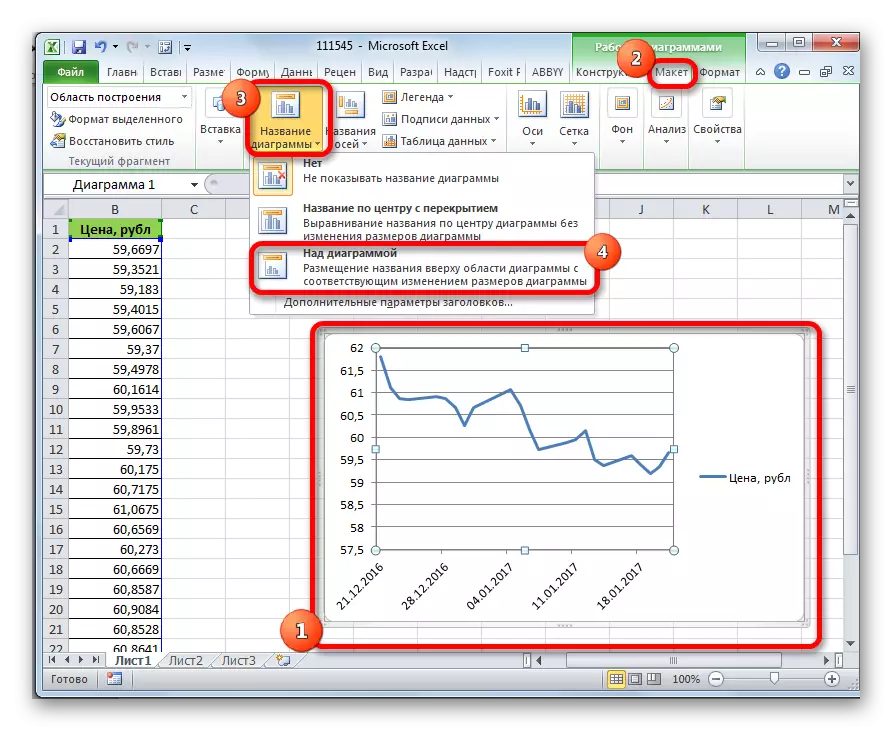
3. After that, the schedule will be built, but it must be further refined. We make the headline of the graph. For this, click on it. In the "Work with Charts" tab that appears, go to the "Layout" tab. In it, click on the "Diagram Title" button. In the list that opens, select the item "above the diagram".



4. In the field that appeared above the schedule, you enter the name that we consider suitable.



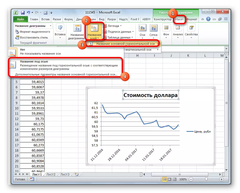
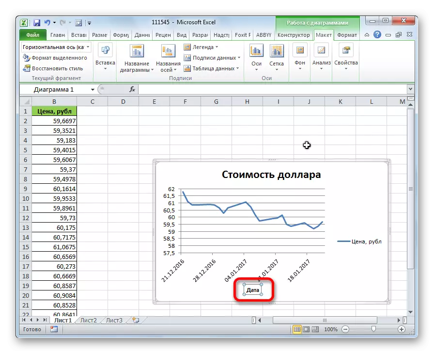
5. Then we sign the axis. In the same tab "Layout", click on the button on the "axis name" tape. Consistently go through the items "name of the main horizontal axis" and "name under the axis".



6. In the field that appears, enter the name of the horizontal axis, according to the context of the data located on it.



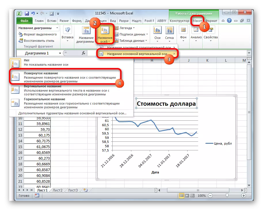
7. In order to assign the name of the vertical axis, we also use the "Layout" tab. Click on the button "name axes". We consistently move on the items of the pop-up menu "Name of the main vertical axis" and "rotated name". This type of axis name location will be most convenient for our type of diagrams.



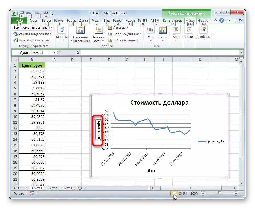
8. In the appeared field of the name of the vertical axis enter the right name.

Lesson: How to make a graph in Excel

Creating a trend line

Now you need to directly add a trend line.

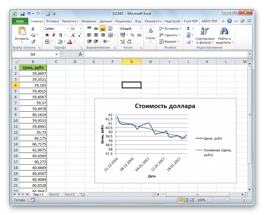
1. Being in the tab "Layout" by clicking on the "Trend Line" button, which is located in the "Analysis" toolbar. From the opening list, choose the item "Exponential approximation" or "linear approximation".



2. After that, the trend line is added to the schedule. By default, it has a black color.

Setting Trend Line

It is possible to further adjust the line.

1. Consistently go to the "Layout" tab on the menu items "Analysis", "Trend Line" and "Additional Trend Line Parameters ...".



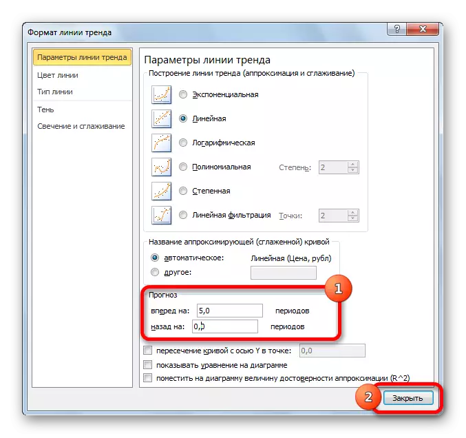
2. The parameters window opens, you can make various settings. For example, you can make a change in the type of smoothing and approximation by selecting one of the six items:
   • Polynomial;
   • Linear;
   • Power;
   • Logarithmic;
   • Exponential;
   • Linear filtration.

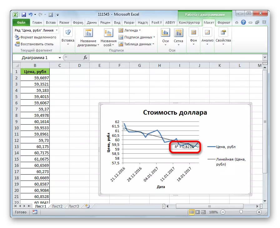
   In order to determine the accuracy of our model, we set a tick about the item "Place the value of the value of the accuracy of the approximation in the diagram." To view the result, click on the "Close" button.

   

   If this indicator is 1, then the model is as reliable as possible. The farther level from one, the less reliability.

If you do not satisfy the level of reliability, you can return again to the parameters and change the type of smoothing and approximation. Then, form a coefficient again.

Forecasting

The main task of the trend line is the ability to compile a forecast for the further development of events.

1. Again, go to the parameters. In the "Forecast" settings block in the appropriate fields, we specify how long or backward periods need to continue the trend line to predict. Click on the "Close" button.



2. Again go to the schedule. It shows that the line is elongated. Now you can determine which approximate indicator is predicted to a specific date while maintaining the current trend.

As you can see, the excel is not difficult to build a trend line. The program provides tools so that it can be configured to be configured to maximize the indicators. Based on the graph, you can make a prognosis for a specific time period.