
The tabulation function is the calculation of the function value for each appropriate argument specified with a specific step in well-established boundaries. This procedure is a tool for solving a variety of tasks. With its help, you can localize the roots of the equation, find highs and minima, solve other tasks. With the Excel program, the tabulation is much easier to perform than using paper, handle and calculator. Let's find out how this is done in this application.
Tabulation use
Tabulization is applied by creating a table in which the value of the argument with the selected step will be recorded in one column, and in the second - the function corresponding to it. Then, on the basis of the calculation, you can build a schedule. Consider how this is done on a specific example.Creating a table
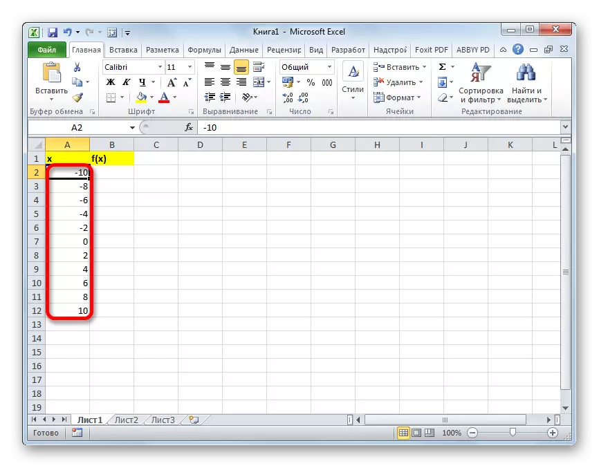
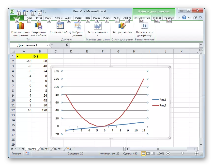
Create a table with a table with columns X, in which the value of the argument will be indicated, and F (x), where the corresponding function is displayed. For example, take the function f (x) = x ^ 2 + 2x, although the function of any kind can be used for the tabulation procedure. We set the step (h) in the amount of 2. The border from -10 to 10. Now we need to fill the argument column, sticking to step 2 at the specified borders.
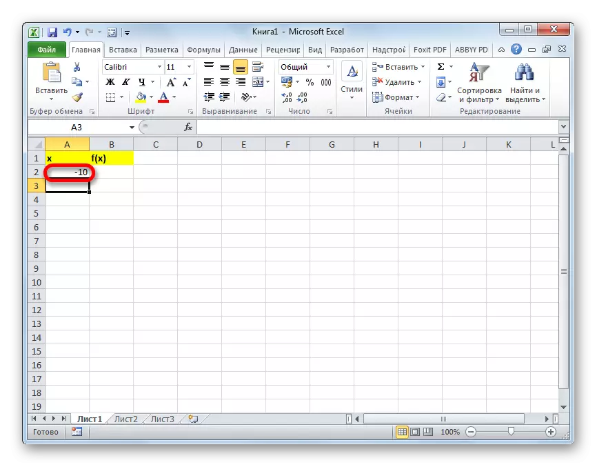
- In the first cell of the column "X" enter the value "-10". Immediately after that we click on the ENTER button. This is very important, since if you try to manipulate the mouse, the value in the cell will turn into a formula, and in this case it is not necessary.
- All further values can be filled by hand, sticking to step 2, but it is more convenient to do this using the autofill tool. Especially this option is relevant if the range of arguments is large, and the step is relatively small.
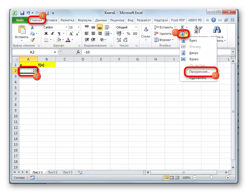
Select the cell containing the value of the first argument. While in the "Home" tab, click on the button "Fill", which is located on the tape in the "Editing" settings block. In the list of action that appears, I choose the clause "Progression ...".
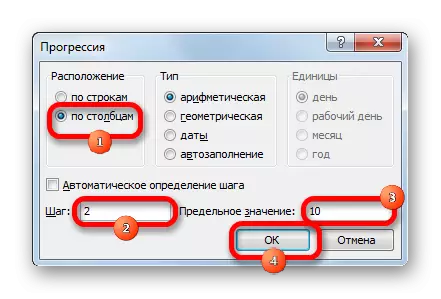
- The progression setting window opens. In the "Location" parameter, we set the switch to the position "by columns", since in our case the values of the argument will be placed in the column, and not in the string. In the "Step" field, set the value 2. In the "Limit value" field, enter the number 10. In order to start the progression, press the "OK" button.
- As you can see, the column is filled with values with a pitch and boundaries.
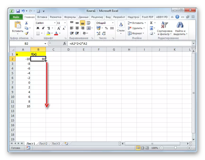
- Now you need to fill the column of the function f (x) = x ^ 2 + 2x. To do this, in the first cell of the corresponding column, write the expression on the following template:
= x ^ 2 + 2 * x
At the same time, instead of the value of X we substitute the coordinates of the first cell from the column with arguments. We click on the ENTER button to display the result of the calculations on the screen.
- In order to calculate the function and in other lines, we will again use the autocomplete technology, but in this case we will apply a fill marker. We establish the cursor to the lower right corner of the cell in which the formula is already contained. The filling marker appears, presented in the form of a small in size of the Cross. Clement the left mouse button and stretch the cursor along the entire column being filled.
- After this action, the entire column with the values of the function will be automatically filled.

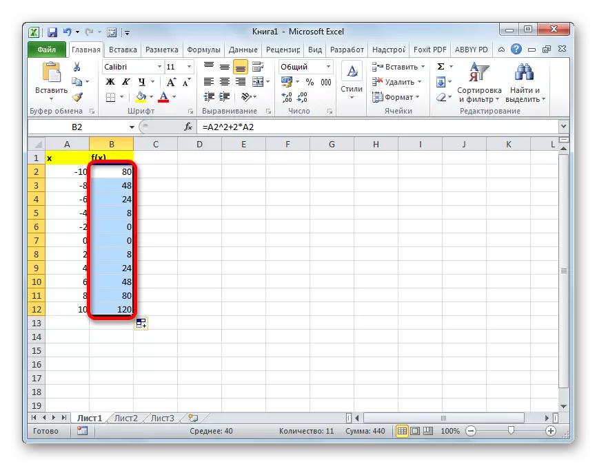
Thus, the tab function was carried out. On its basis, we can find out, for example, that at least the function (0) is achieved with the values of the argument -2 and 0. Maximum function within the boundaries of the argument variation from -10 to 10 is achieved at a point corresponding to the argument 10, and is 120.
Lesson: How to make auto-filling in Excel
Building graphics
Based on the tabulated tab in the table, you can build a function schedule.
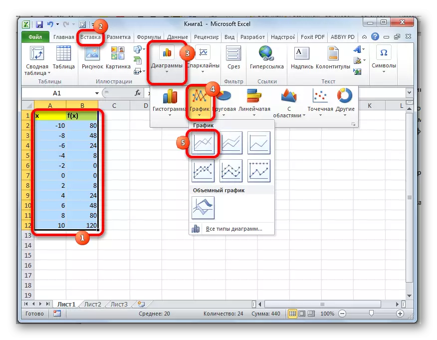
- Select all the values in the table with the cursor with the left mouse button. Let us turn to the "Insert" tab, in the chart tool block on the tape we press the "Graphs" button. A list of available graphics options is available. Choose the type that we consider the most suitable. In our case, it is perfect, for example, a simple schedule.
- After that, the program software performs the procedure for constructing a graph based on a selected table range.
Further, if desired, the user can edit the chart as it seems necessary using Excel tools for these purposes. You can add the names of the axes of coordinates and graphics as a whole, remove or rename the legend, remove the argument line, etc.
Lesson: How to build a schedule in Excel
As we see, the tabulation function, in general, the process is simple. True, calculations may take quite a long time. Especially if the boundaries of the arguments are very broad, and the step is small. Significantly saved the time to help the Excel auto-complete tools. In addition, in the same program, on the basis of the result, you can build a graph for a visual presentation.