Interpolation in Excel: 3 work options

It happens when in the array of well-known values ​​you need to find intermediate results. In mathematics, this is called interpolation. In Excel, this method can be applied both for tabular data and to build graphs. We will analyze each of these ways.

Use of interpolation

The main condition in which interpolation can be applied is that the desired value should be inside the data array, and not go beyond its limit. For example, if we have a set of arguments 15, 21 and 29, then when you find a function for argument 25, we can use interpolation. And to search for the appropriate value for the argument 30 - no longer. This is the main difference between this procedure from extrapolation.

Method 1: Interpolation for tabular data

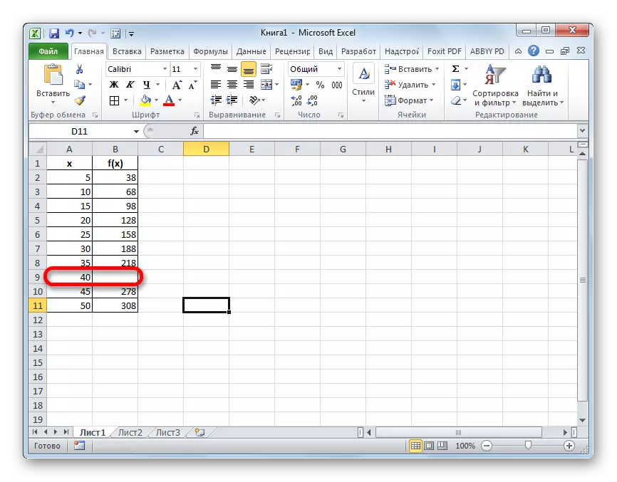
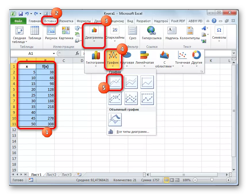
First of all, consider the use of interpolation for the data that are located in the table. For example, take an array of arguments and corresponding to them values ​​of the function, the ratio of which can be described by a linear equation. This data is posted in the table below. We need to find the appropriate function for argument 28. Make it is the easiest way with the help of a prediction operator.

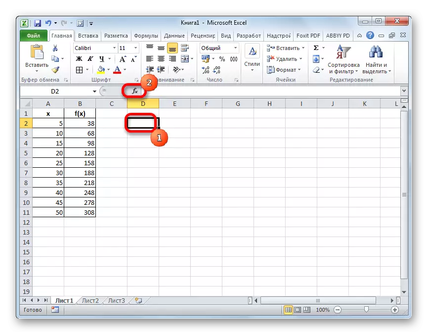
1. We highlight any empty cell on the sheet where the user plans to output the result from the actions taken. Next, click on the "Insert function" button, which is placed on the left of the formula row.



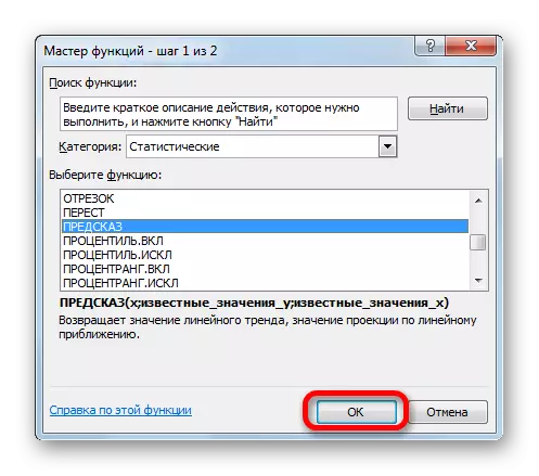
2. The functions wizard window is activated. In the category "Mathematical" or "full alphabetical list" we are looking for the name "Predict". After the corresponding value is found, we highlight it and click on the "OK" button.



3. The predicted function arguments window starts. It has three fields:
   • X;
   • Known values ​​y;
   • Known values ​​x.

   In the first field, we simply need manually from the keyboard to drive the values ​​of the argument, the function of which should be found. In our case, it is 28.

   In the "Known R values" field, you need to specify the coordinates of the table range in which the values ​​of the function are contained. This can be done manually, but it is much easier and more convenient to set the cursor in the field and select the appropriate area on the sheet.

   Similarly, set the coordinates of the arguments with arguments in the "Known Values ​​X" field.

   After all the necessary data is entered, press the "OK" button.



4. The desired function of the function will be displayed in the cell that we allocated in the first step of this method. The result was the number 176. It is precisely it will be the result of the interpolation procedure.

Lesson: Master of Functions in Excel

Method 2: Interpolation of the schedule using its settings

The interpolation procedure can also be applied when building a function graphs. It is relevant if the chart is based on the table, on the basis of which the corresponding function is not specified to one of the arguments, as in the image below.

1. We carry out the construction of the graph by the usual method. That is, being in the "Insert" tab, allocate a table range based on which the construction will be conducted. Click on the "Schedule" icon, placed in the chart toolbar. From the list of graphs that appears, choose the one that we consider more appropriate in this situation.



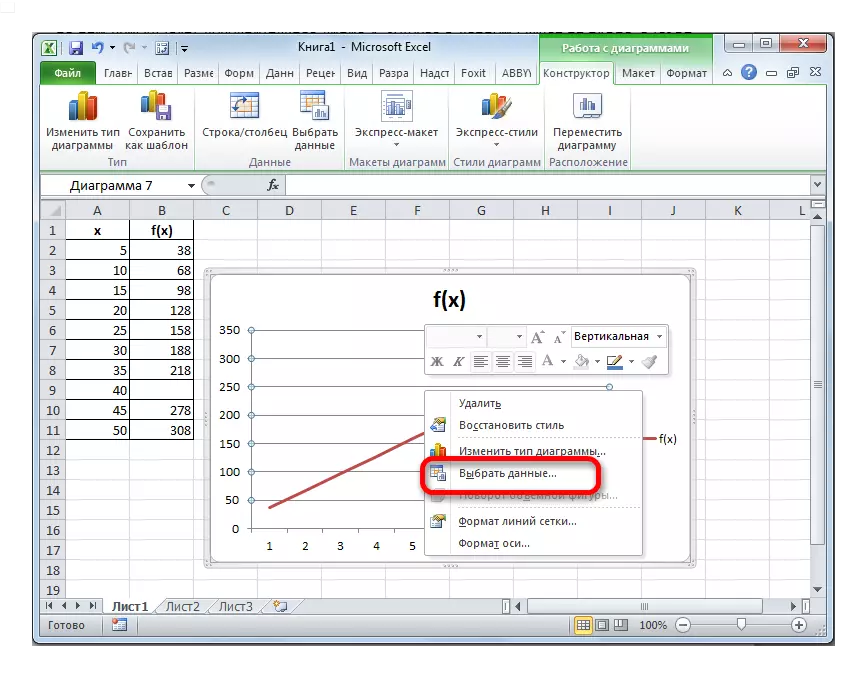
2. As you can see, the schedule is built, but not quite in this form, as we need. First, it is broken, since for one argument there was no appropriate function. Secondly, it presents an additional line X, which in this case is not needed, as well as on the horizontal axis, simply points are indicated in order, and not the values ​​of the argument. Let's try to fix it all.

   To begin with, we highlight a solid blue line that you want to remove and press the DELETE button on the keyboard.



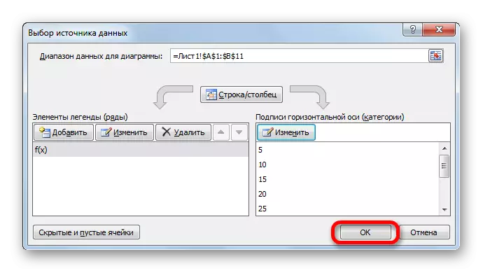
3. We highlight the entire plane on which the schedule is located. In the context menu that appears, click on the "Select data ..." button.



4. The data source selection window is launched. In the right block of "signature of the horizontal axis" we click on the "Change" button.



5. A small window opens, where you need to specify the coordinates of the range, the values ​​from which will be displayed on the horizontal axis scale. Install the cursor in the "range of signature range" field and sim sim simply select the corresponding area on the sheet in which the function arguments are contained. Click on the "OK" button.



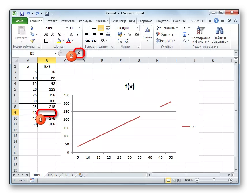
6. Now we have to fulfill the main task: with the help of interpolation eliminate the gap. Returning to the window for selecting the data range, click on the "Hidden and Empty Cells" button located in the lower left corner.



7. The settings window of hidden and empty cells opens. In the "Show empty cells" parameter, set the switch to the "line" position. Click on the "OK" button.



8. After returning to the source selection window, confirm all the changes made by clicking the "OK" button.

As you can see, the graph is adjusted, and the gap by interpolation is removed.

Lesson: How to build a schedule in Excel

Method 3: Interpolation of the graph using the function

You can also interporate graphics using a special ND function. It returns indefinite values ​​to the specified cell.

1. After the schedule is built and edited, as you need, including the correct distribution of the Signature of the scale, it remains only to eliminate the gap. Select a blank cell in the table from which the data is tightened. We click on the already familiar to us "Insert function" icon.



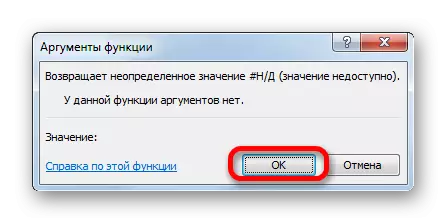
2. Wizard opens. In the category "Check properties and values" or "Full Alphabetical List" we find and highlight the entry "ND". Click on the "OK" button.



3. This function does not have an argument, as reported by the information window that appears. To close it simply click on the "OK" button.



4. After that, the validity of the "# H / D" error appeared in the selected cell, but how can you observe, the scope of the schedule was automatically eliminated.

It can be done even easier, not running a master of functions, but simply from the keyboard to drive into an empty cell value "# H / D" without quotes. But it already depends on what user is more convenient.

As you can see, in the Excel program you can perform interpolation as tabular data using the predicted function and graphics. In the latter case, it is feasible using the graphics settings or the use of the ND function that causes the "# H / D" error. The choice of which method is to use depends on the setting of the problem, as well as the personal preferences of the user.