Transposing matrices in Excel

When working with matrices, sometimes you need to transpose them, that is, speaking with simple words, turn over. Of course, you can convert data manually, but Excel offers several ways to do it easier and faster. Let's analyze them in detail.

Transposing process

Transposing the matrix is ​​the process of changing columns and lines in places. The Excel program has two possible transposition features: using the TRAC function and using a special insert tool. Consider each of these options in more detail.

Method 1: TransP operator

The TRAC function refers to the category of "Links and Arrays" operators. A feature is that she has, as in other functions working with arrays, the result of issuing is not the content of the cell, but a whole data array. The syntax of the function is quite simple and looks like this:

= TRACP (array)

That is, the only argument of this operator is a reference to an array, in our case the matrix that should be converted.

Let's see how this function can be applied by an example with a real matrix.

1. We highlight a blank cell on the sheet, planned to make an extremely upper left cell of the converted matrix. Next, click on the "Insert function" icon, which is located near the formula row.



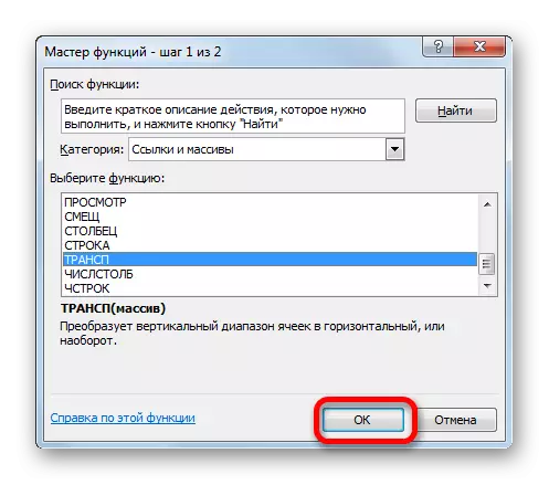
2. Running the wizard of functions. Open in it the category "Links and arrays" or "Full alphabetical list". After the name "TRACT" was found, produce its allocation and press the "OK" button.



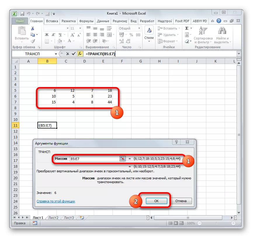
3. The TRACE function arguments window starts. The only argument of this operator corresponds to the "Array" field. It is necessary to make the coordinates of the matrix, which should be turned over. To do this, set the cursor in the field and, by holding the left mouse button, we highlight the entire range of the matrix on the sheet. After the address of the area is displayed in the argument window, click on the "OK" button.



4. But, as we see, in a cell, which is intended to display the result, the incorrect value is displayed as an error "# mean!". This is due to the features of the work of arrays. To correct this error, select the range of cells in which the number of rows should be equal to the number of columns of the initial matrix, and the number of columns - the number of rows. Such a match is very important for the result to be displayed correctly. At the same time, the cell containing an expression "# mean!" It must be the upper left cell of the array allocated and it is from it that you should start the selection procedure by closing the left mouse button. After you have selected, set the cursor in the formula string immediately after the expression of the TransP operator, which should be displayed in it. After that, to make a calculation, you need to press the ENTER button, as is customary in conventional formulas, and to dial a Ctrl + Shift + Enter combination.



5. After these actions, the matrix was displayed as we need, that is, in a transposed form. But there is another problem. The fact is that now the new matrix is ​​an array associated formula that cannot be changed. When trying to make any change with the contents of the matrix will pop up an error. Some users such a state of affairs quite satisfies, as they are not going to make changes in the array, but others need a matrix with which you can fully work.

   To solve this problem, we allocate the entire transposed range. By moving into the "Home" tab, click on the "Copy" icon, which is located on the ribbon in the clipboard group. Instead of the specified action, you can, after the selection, make a set of a standard keyboard shortcut to copy Ctrl + C.



6. Then, without removing the selection from the transposed range, make the click on it with the right mouse button. In the context menu in the Insert Parameters group, click on the "Value" icon, which has a view of the pictogram with the image of numbers.

   

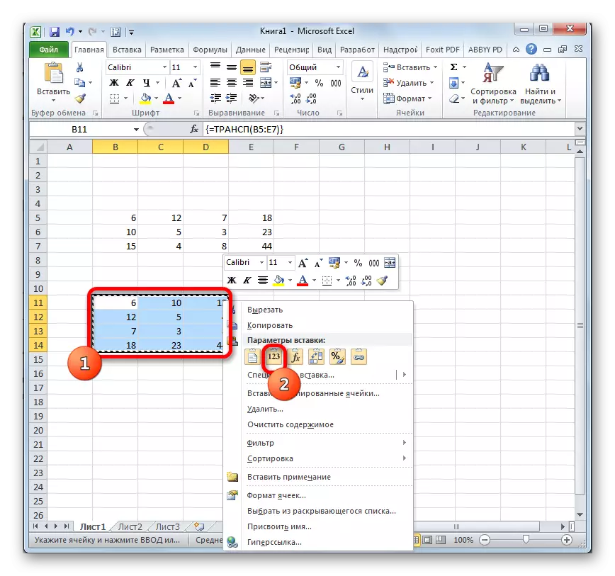
   Following this, the massif formula of the TRAC will be removed, and in cells only the values ​​can remain with which you can work in the same way as with the original matrix.

Lesson: Master of Functions in Excel

Method 2: Transposing the matrix using a special insertion

In addition, the matrix can be transposed using one context menu item that is called "Special Insert".

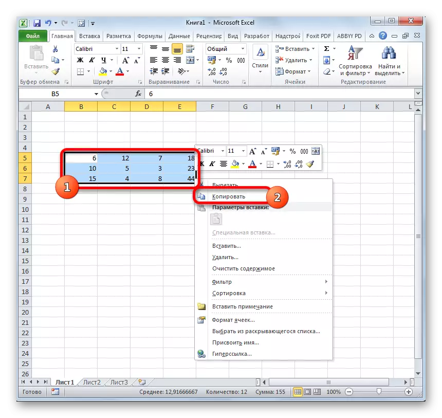
1. Select the source matrix with the cursor by holding the left mouse button. Next, by clicking on the "Home" tab, click on the "Copy" icon, located in the "Exchange buffer" settings block.

   

   Instead, you can do differently. Having selecting the area by clicking on it right mouse button. The context menu is activated, in which you should select "Copy".

   

   In the form of an alternative to two previous copy options, you can, after selecting, make a set of a combination of hot keys Ctrl + C.

2. We choose a blank cell on the sheet, which should be an extreme upper left element of a transposed matrix. We click on it right-click. Following this, the context menu is activated. It is moving on the "Special Insert" item. Another small menu appears. It also has a paragraph called "Special Box ...". Click on it. You can also select the selection, instead of calling the context menu, dial a Ctrl + Alt + V combination on the keyboard.



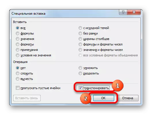
3. A special insert window is activated. There are many options for choosing, exactly how to insert previously copied data. In our case, you need to leave almost all default settings. Only around the transpose parameter should be installed. Then you need to click on the "OK" button, which is located at the bottom of this window.



4. After these actions, the transposed matrix will be displayed in a predetermined part of the sheet. Unlike the previous way, we have already received a full-fledged matrix, which can be changed, like the source. No further refinement or transformation is required.



5. But if you wish, if the initial matrix you do not need it, you can delete it. To do this, highlight it with its cursor by holding the left mouse button. Then click on the dedicated right-click item. In the context menu, which will open after this, select the "Clear Content" item.

After these actions, only the converted matrix will remain on the sheet.

These two ways, which were discussed above, you can transpose in Excel not only the matrices, but also full-fledged tables. The procedure will be almost identical.

Lesson: How to flip the table in exile

So, we found out that in the Excel program, the matrix can be transposed, that is, turn over, changing columns and lines by places, in two ways. The first option involves the use of the Function of the TRACP, and the second - the tools of a special insert. By and large, the final result, which is obtained when using both of these methods, is no different. Both methods work in almost any situation. So when choosing a transformation option, personal preferences of a particular user are on the fore. That is, which of these methods is more convenient for you more convenient, and use.