How to Show Hidden Cells in Excel

When working with Excel tables, sometimes you need to hide formulas or temporarily unnecessary data so that they do not interfere. But sooner or later, the moment comes when it is necessary to adjust the formula, or the information that is contained in the hidden cells, it is suddenly needed to the user. Then it becomes relevant to how to display hidden items. Let's find out how to solve this task.

Display enable procedure

Immediately, it must be said that the choice of the option to turn on the display of hidden elements primarily depends on how they were hidden. Often these methods use completely different technology. There are such options to hide the contents of the sheet:

• shift boundaries of columns or strings, including through the context menu or the button on the tape;
• grouping data;
• filtration;
• Hiding the contents of cells.

Now let's try to figure out how you can display the contents of the elements hidden using the above methods.

Method 1: Border opening

Most often, users hide columns and strings, bow their borders. If the boundaries were shifted very tightly, then it's hard to cling to the edge to push them back. Find out how it can be done easily and quickly.

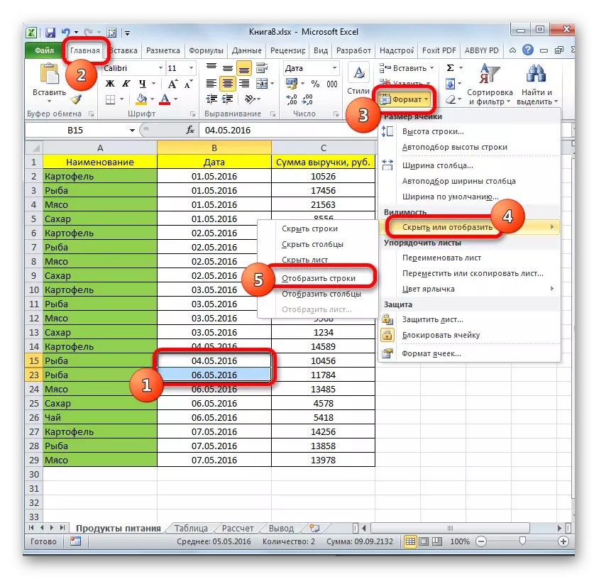
1. Select two adjacent cells, between which there are hidden columns or strings. Go to the "Home" tab. Click on the "Format" button, which is located in the "Cell tools" block. In the list that appears, we bring the cursor to the item "Hide or Display", which is in the "Visibility" group. Next, in the menu that appears, select the "Display strings" or "Display columns" item, depending on what is hidden.



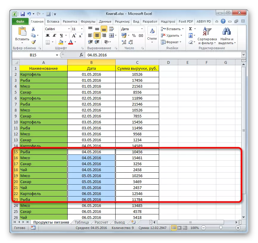
2. After this action, hidden elements will seem on the sheet.

There is another option that can be used to display hidden by shifting the boundaries of elements.

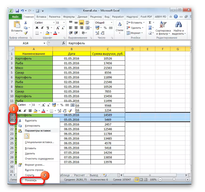
1. On the horizontal or vertical coordinate panel, depending on what is hidden, columns or strings, with a cursor with the left mouse button, we highlight two adjacent sectors, between which the elements are hidden. Click on highlighting the right mouse button. In the context menu, select "Show".



2. Hidden items will be immediately displayed on the screen.

These two options can be applied not only if the borders of the cell were shifted manually, but also if they were hidden using the tools on the ribbon or the context menu.

Method 2: Lump

Lines and columns can also be hidden using a grouping when they are collected in separate groups, and then hidden. Let's see how to display them on the screen again.

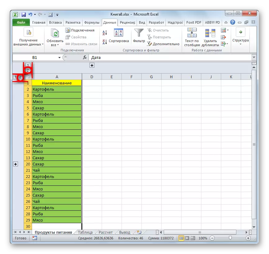
1. An indicator that strings or columns are grouped and hidden is the presence of the "+" icon to the left of the vertical coordinate panel or on top of the horizontal panel, respectively. In order to show the hidden items, just click on this icon.

   

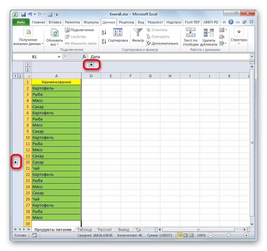
   You can also display them by clicking on the last digit numbering of groups. That is, if the last digit is "2", then click on it, if "3", then click on this figure. A specific number depends on how many groups are invested in each other. These numbers are located on top of the horizontal coordinate panel or to the left of the vertical.



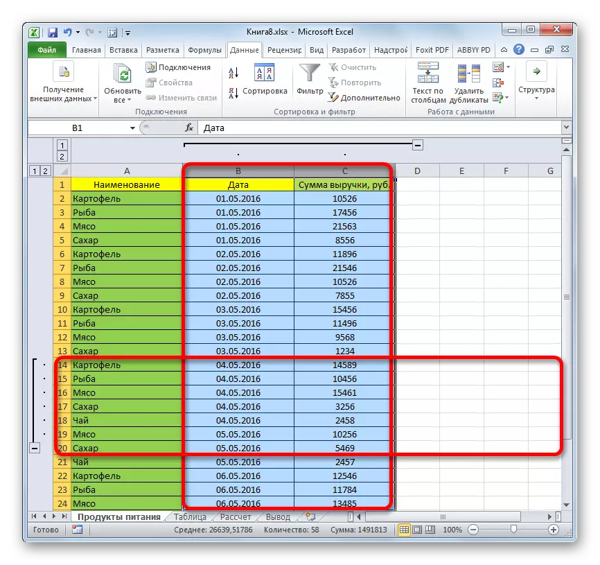
2. After any of these actions, the contents of the group will open.



3. If this is not enough for you and you need to make full unloading, then first select the corresponding columns or lines. Then, being in the "Data" tab, click on the "Ungroup" button, which is located in the "Structure" block on the tape. Alternatively, you can press the combination of hot shift + alt + arrow left buttons.

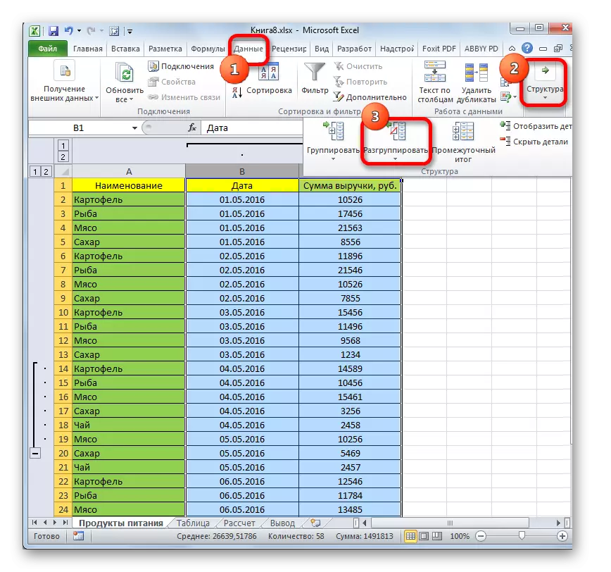
Groups will be deleted.

Method 3: Removing the filter

In order to hide temporarily unnecessary data, filtering is often used. But when it comes to return to work with this information, the filter needs to be removed.

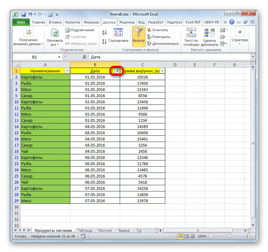
1. Click on the filter icon in the column, by the values ​​of which filtering was performed. Such columns find easily, since they have an ordinary filter icon with an inverted triangle is complemented by another icon in the form of watering.



2. The filtering menu opens. Install the ticks opposite those points where they are absent. These lines are not displayed on the sheet. Then click on the "OK" button.



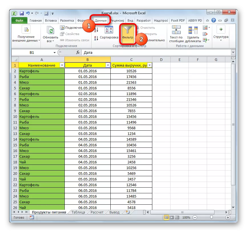
3. After this, the row will appear, but if you want to remove filter at all, you need to click on the "Filter" button, which is located in the Data tab on the tape in the Sort and Filter group.

Method 4: Formatting

In order to hide the contents of individual cells, formatting is introduced by entering the expression ";;;" in the format field. To show the hidden content, you need to return the original format to these elements.

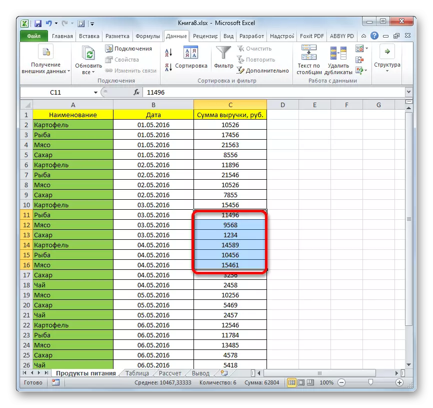
1. Select cells in which hidden content is located. Such elements can be determined by the fact that no data is displayed in the cells themselves, but when they are selected, the contents will be shown in the formula string.



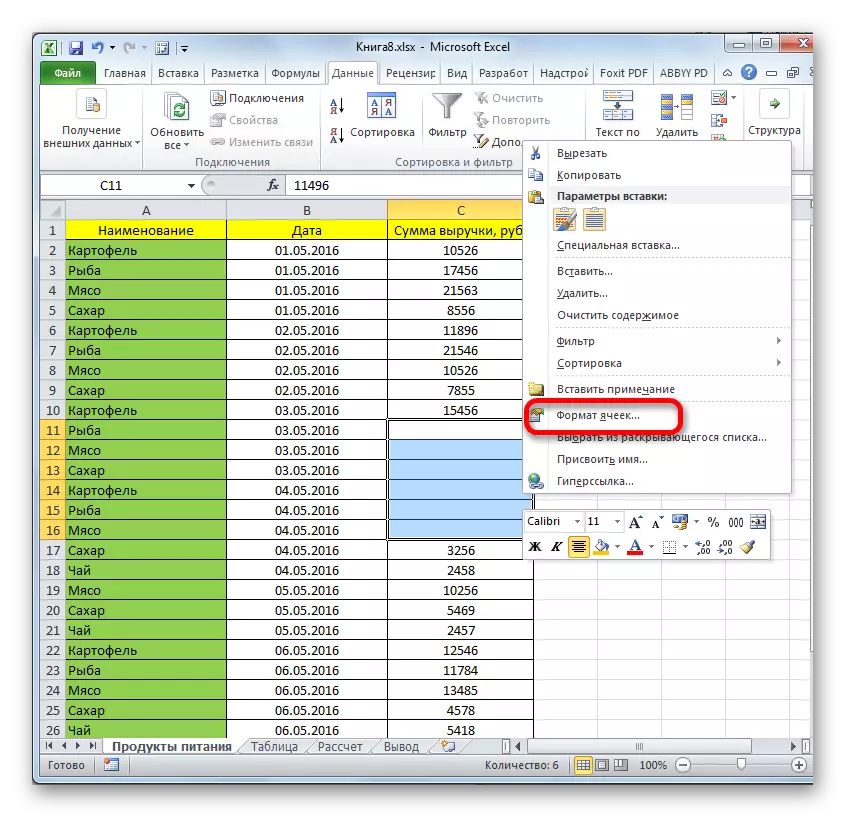
2. After the selection was made, click on it with the right mouse button. The context menu is launched. Select the item "Format cells ..." by clicking on it.



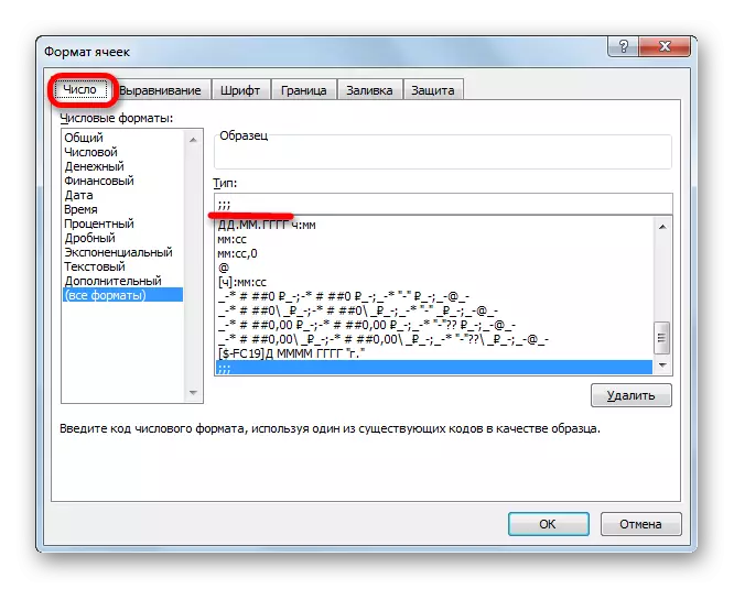
3. The formatting window is started. We make moving into the "Number" tab. As you can see, the "Type" field displays the value ";;;".



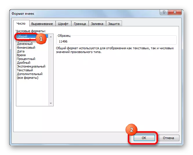
4. Very good if you remember what was the initial formatting of the cells. In this case, you will only remain in the "Numeric formats" parameters block to highlight the corresponding item. If you do not remember exact format, then rely on the essence of the content, which is located in the cell. For example, if there is information about time or date there, choose the "Time" or "date" item, and the like. But for most types of content, the "General" item is suitable. We make a choice and click on the "OK" button.

As you can see, after that, hidden values ​​are displayed again on the sheet. If you consider that displaying information incorrectly, and, for example, instead of the date you see the usual set of numbers, then try to change the format again.

Lesson: How to change cell format in Excel

When solving the problem of displaying hidden elements, the main task is to determine which technology they were hidden. Then, based on this, apply one of those four ways that were described above. It is necessary to understand that if, for example, the content was hidden by closing the boundaries, then the dismissal or removal of the filter cannot be displayed.