Function Mother in Excel

As you know, Excel has many tools for working with matrices. One of them is the Muffer function. With this operator, users appear to multiply different matrices. Let's find out how to use this feature in practice, and what is the main nuances of working with it.

Using the Muffer operator

The main task of the mum comes, as mentioned above, is to multiply two matrices. It refers to the category of mathematical operators.

The syntax of this feature is as follows:

= Mother (array1; array2)

As we see, the operator has only two arguments - "array1" and "array". Each of the arguments is a reference to one of the matrices, which should multiply. This is exactly what the operator specified above.

An important condition for the application of mums is that the number of strings of the first matrix should coincide with the number of columns of the second. In the opposite case, an error will be issued as a result of processing. Also, in order to avoid an error, none of the elements of both arrays should be empty, and they must fully consist of numbers.

Matrix multiplication

Now let's consider on a specific example, as you can multiply two matrices, applying the Muffer operator.

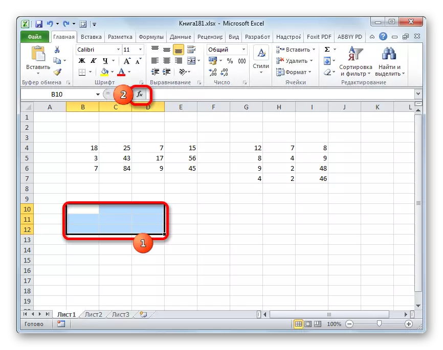
1. Open the Excel sheet on which two matrices are already located. We highlight an area of ​​empty cells on it, which horizontally has in its composition the number of strings of the first matrices, and vertically the number of columns of the second matrix. Next, we click on the "Insert function" icon, which is located near the line of formulas.



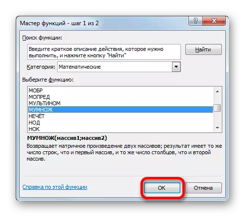
2. The functions wizard starts. We should go to the category "Mathematical" or "Full Alphabetical List". In the list of operators, it is necessary to find the name "Muffer", highlight it and click on the "OK" button, which is located at the bottom of this window.



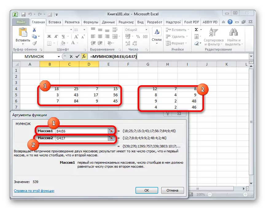
3. The window of the arguments of the operator mumbette is launched. As we see, it has two fields: "array1" and "array". In the first one must specify the coordinates of the first matrix, and in the second, respectively, the second. In order to do this, set the cursor in the first field. Then we produce clamp with the left mouse button and select the area of ​​the cells containing the first matrix. After performing this simple procedure, the coordinates will be displayed in the selected field. A similar action is carried out with the second field, only this time, by holding the left mouse button, we highlight the second matrix.

   After the addresses of both matrices are recorded, do not rush to press the "OK" button, placed in the lower part of the window. The fact is that we are dealing with the function of the array. It provides that the result is not displayed in one cell, as in conventional functions, but immediately into a whole range. Therefore, to output the data processing, using this operator, it is not enough to press the Enter key, placing the cursor in the formula row, or click on the "OK" button while in the argument window of the function that is currently open at the moment. You need to apply pressing the CTRL + SHIFT + ENTER key combination. We carry out this procedure, and the "OK" button does not touch.



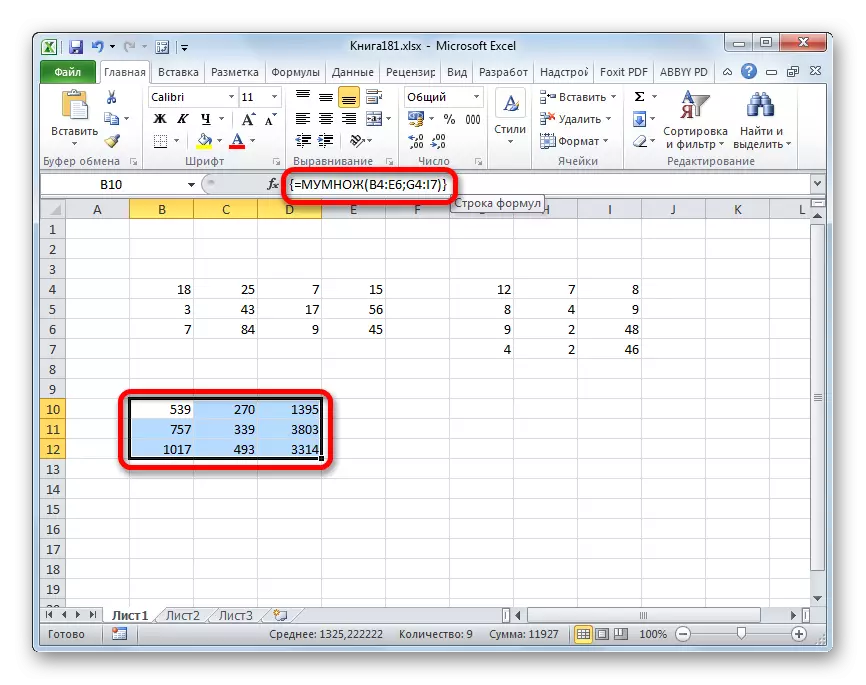
4. As we can see, after pressing the specified keyboard combination, the arguments of the operator's arguments, the mumset closed, and the range of the cells, which we allocated in the first step of this instruction, was filled with data. It is these values ​​that are the result of multiplying one matrix to another, which performed the Muffer operator. As we see, in the formula row, the function is taken in curly brackets, which means its belonging to operators of arrays.



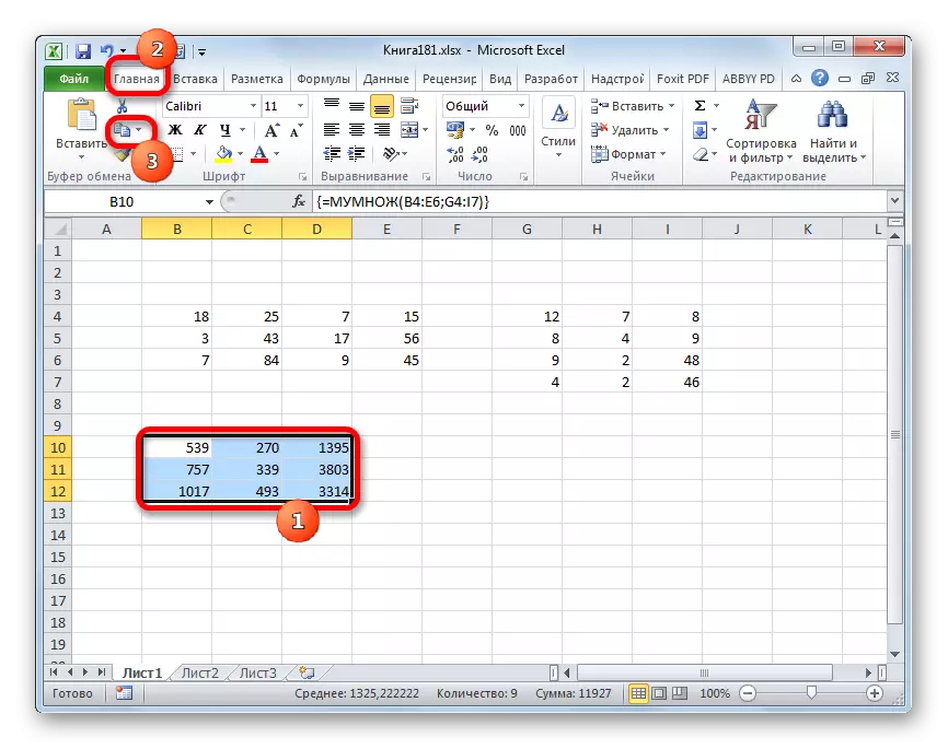
5. But it is precisely that the result of processing the function to mums is a solid array, prevents its further change if necessary. When you try to change any of the numbers of the user's final result, it will be waiting for a message that informs that it is impossible to change the part of the array. To eliminate this inconvenience and convert a unchanging array to a normal range of data with which you can work, carry out the following steps.

   We highlight this range and, while in the Home tab, click on the "Copy" icon, which is located in the "Exchange Buffer" toolbar. Also, instead of this operation, you can apply the CTRL + C key set.



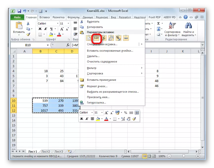
6. After that, without removing the selection from the range, click on it with the right mouse button. In the opened context menu in the "Insert Settings" block, select the "Values" item.



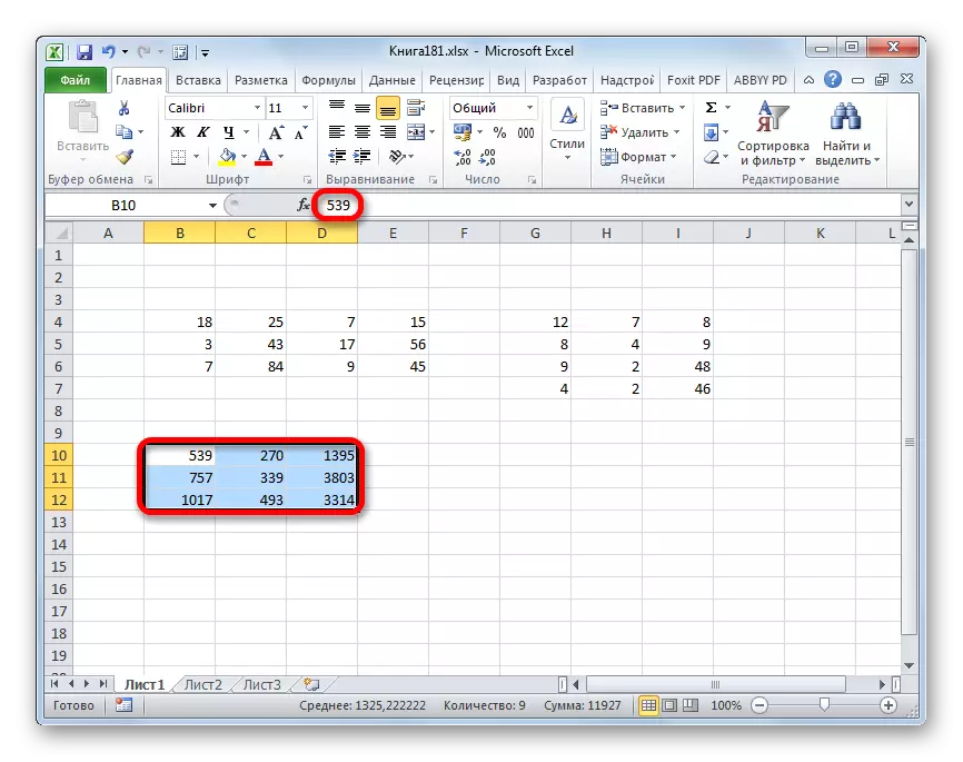
7. After performing this action, the final matrix will no longer be presented as a single inextive range and it can be done with various manipulations.

Lesson: Work with arrays in Excel

As you can see, the mum's operator allows you to quickly and easily multiply in the excel two matrices on each other. The syntax of this function is quite simple and users should not have problems with entering data into the argument window. The only problem that may occur when working with this operator lies in the fact that it represents the function of the array, and therefore has certain features. To display the result, it is necessary to pre-select the corresponding range on the sheet, and then after entering the arguments to calculate, apply a special key combination, designed to work with such a type of data - Ctrl + Shift + Enter.