EXCEL Function Function

In some cases, the user is faced with the task to return a certain number of characters from another cell from another cell, starting from the specified sign on the left. With this task, the PSTR function perfectly copes. Its functional increases even more if other operators are used in combination with it, such as search or find. Let's look more in more detail what the capabilities of the PSTR function are and see how it works on specific examples.

Using the PST

The main task of the PSTr operator is to remove from the specified element of a sheet of a certain number of printed signs, including spaces, starting from the indicated on the left of the symbol. This feature refers to the category of text operators. Its syntax takes the following form:

= PST (text; initial_position; number_names)

As we see, this formula consists of three arguments. All of them are mandatory.

The "Text" argument contains the address of the leaf element in which the text expression is located with removable signs.

The initial position argument is presented in the form of a number that indicates which sign on the account, starting on the left, needs to be extracted. The first sign is considered "1", the second for "2", etc. Even gaps are taken into account in the calculation.

The argument "Number of Signs" contains a number of characters in itself, ranging from the initial position to be removed into the target cell. When calculating the same way as the previous argument, gaps are taken into account.

Example 1: Single Removal

Describe the examples of the use of the Pastro function to start from the simplest case when it is necessary to extract a single expression. Of course, such options in practice are extremely rare, so we give this example only as familiarization with the principles of the specified operator.

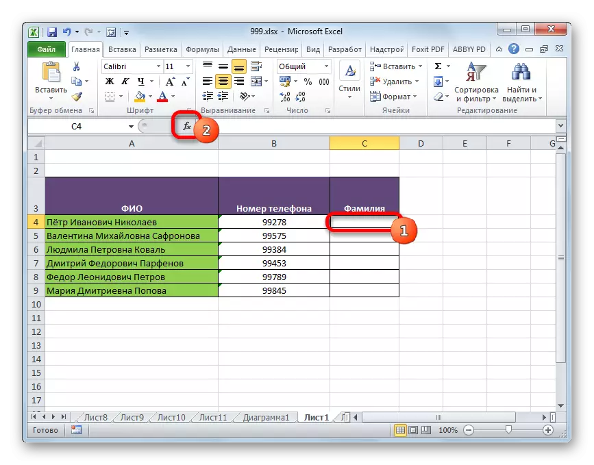
So, we have a table of employees of the enterprise. The first column shows the names, surnames and patronymic officers. We needed using the PSTR operator to extract only the name of the first person from the list of Peter Ivanovich Nikolaev in the specified cell.

1. Select the sheet element in which it will be extracted. Click on the "Insert function" button, which is located near the formula row.



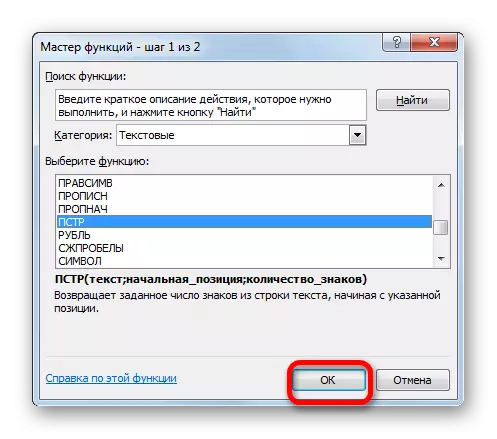
2. The functions wizard window starts. Go to the category "Text". We allocate the name "PST" and click on the "OK" button.



3. The "PSTR" operator arguments window launch. As you can see, in this window the number of fields corresponds to the number of arguments of this function.

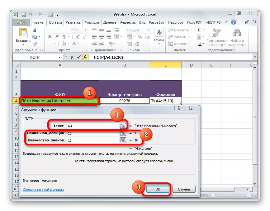
   In the field "Text" we introduce the coordinates of the cell, which contains the names of workers. In order not to drive the address manually, we simply install the cursor in the field and click the left mouse button on the element on the sheet in which the data we need are contained.

   In the "Starting Position" field, you need to specify the character number, counting on the left, from which the name of the employee begins. When calculating, we also consider spaces. The letter "H", with which the name of the employee of Nikolaev begins, is the fifteenth symbol. Therefore, in the field, we set the number "15".

   In the "Number of Signs" field, you need to specify the number of characters from which the surname consists. It consists of eight characters. But given that after the surname, there are no more characters in the cell, we can indicate a larger number of characters. That is, in our case, you can put any number that is equal to or more eight. We put, for example, the number "10". But if after the surname, there would be more words, numbers or other characters in the cell, then we would have to install only the exact number of signs ("8").

   After all the data is entered, press the "OK" button.



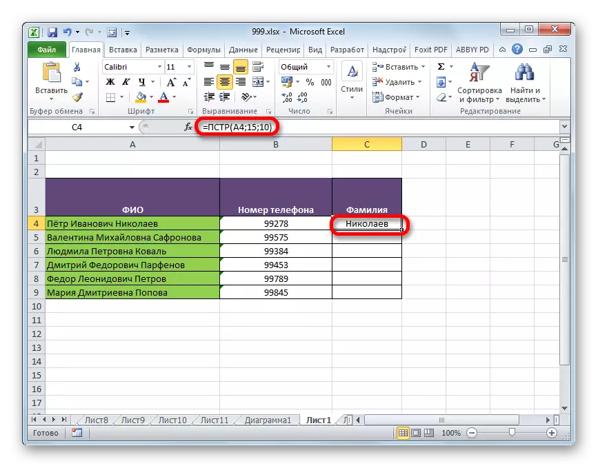
4. As we see, after this action, the name of the employee was displayed in the example 1 specified in the first step.

Lesson: Master of Functions in Excel

Example 2: Group Extraction

But, of course, for practical purposes it is easier to manually drive a single surname than to apply for this formula. But to transfer the data group, the use of the function will be quite appropriate.

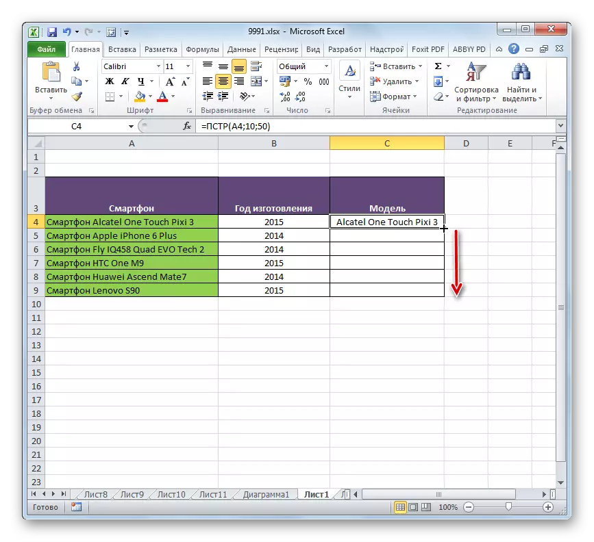
We have a list of smartphones. Before the name of each model is the word "smartphone". We need to make a separate column only the names of the models without this word.

1. We highlight the first empty element of the column to which the result will be displayed, and call the arguments window of the PSTR operator in the same way as in the previous example.

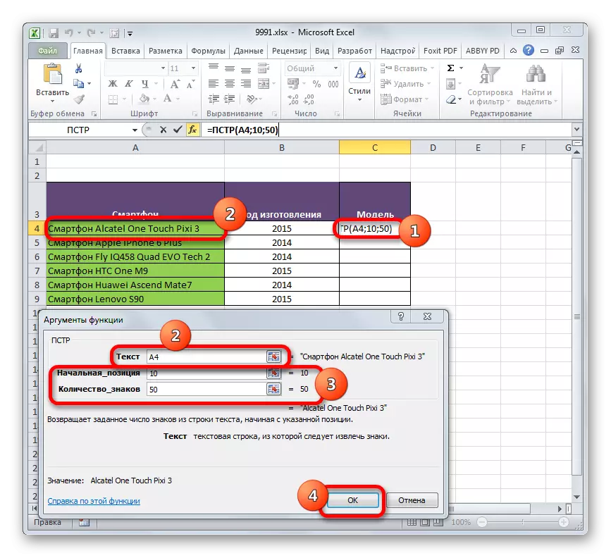
   In the "Text" field, specify the address of the first column element with the source data.

   In the "Starting Position" field, we need to specify the character number starting from which the data will be retrieved. In our case, in each cell before the name of the model, the word "smartphone" and a space. Thus, the phrase that needs to be brought into a separate cell everywhere starts from the tenth symbol. Install the number "10" in this field.

   In the "Number of Signs" field, you need to set the number of characters that contains the output phrase. As we see, in the name of each model, a different number of characters. But the situation saves the fact that after the name of the model, the text in the cells ends. Therefore, we can set any number in this field that is equal to or more than the number of characters in the longest name in this list. We establish an arbitrary number of "50" signs. The name none of the listed smartphones does not exceed 50 characters, so the specified option is suitable for us.

   After the data is entered, press the "OK" button.



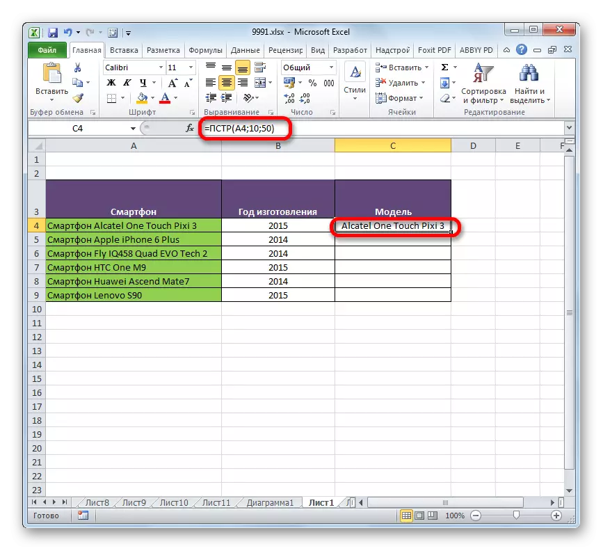
2. After that, the name of the first model of the smartphone is displayed in a predetermined cell of the table.



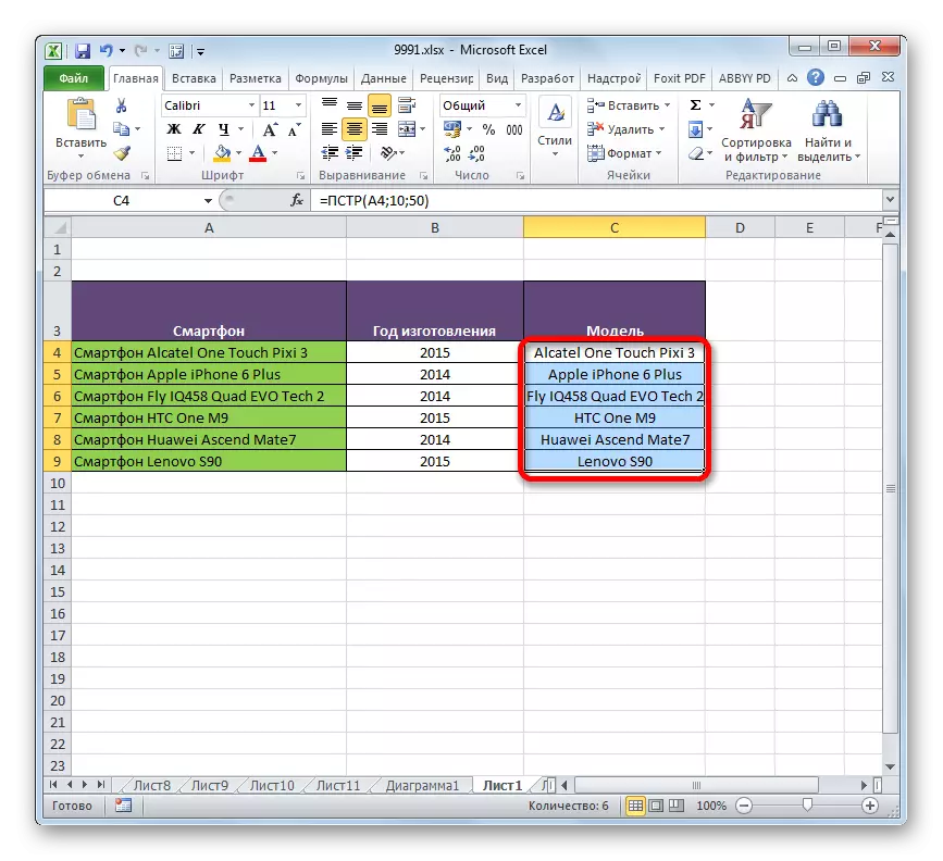
3. In order not to enter the formula in each cell to each cell separately, make it copying it by filling marker. To do this, put the cursor to the lower right corner of the cell with the formula. The cursor is converted to the fill marker in the form of a small cross. Click the left mouse button and pull it to the very end of the column.



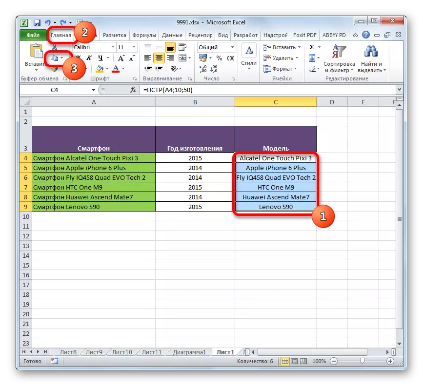
4. As you can see, the entire column will after that will be filled with the data we need. The secret is that the "Text" argument is a relative reference and as the position of the target cells changes also change.



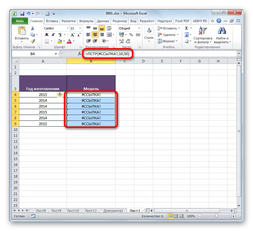
5. But the problem is that if we decide to suddenly change or remove a column with initial data, then the data in the target column will be displayed incorrectly, as they are connected with each other formula.

   

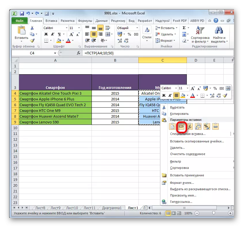
   To "untie" the result from the original column, produce the following manipulations. Select a column that contains a formula. Next, go to the "Home" tab and click on the "Copy" icon, located in the "Buffer" on the tape.

   

   As an alternative action, you can download the CTRL + C key combination after the selection.

6. Next, without removing the selection, click on the column with the right mouse button. The context menu opens. In the "Insert Parameters" block, click on the "Value" icon.



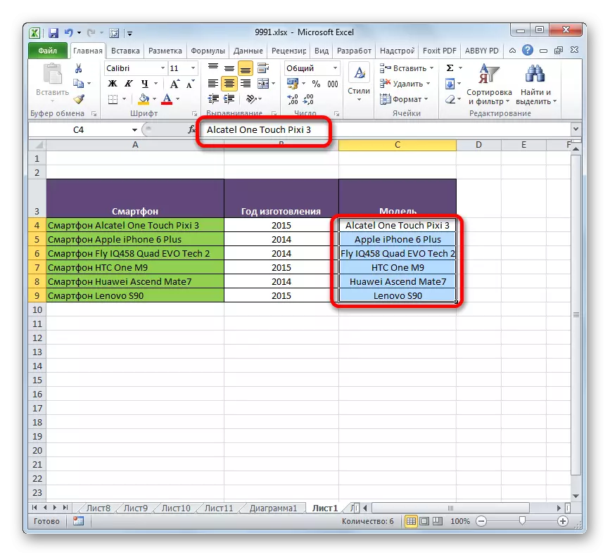
7. After that, instead of formulas, values ​​will be inserted into the selected column. Now you can change or delete the source column without fears. It will not affect the result.

Example 3: Using the combination of operators

But still, the above example is limited to the fact that the first word in all source cells should have an equal number of characters. Application Together with the function of the PSTR operators, the search or find will allow you to significantly expand the possibilities of using the formula.

Text operators Search and find return the position of the specified symbol in the text viewed.

Syntax function Search Next:

= Search (desired_text; Text_D_Poe; initial_position)

The operator's syntax looks like:

= Find (desired_text; viewed_text; nach_Position)

By and large, the arguments of these two functions are identical. Their main difference is that the search operator during data processing does not take into account the letters register, and find it takes into account.

Let's see how to use the search operator in combination with the PSTR function. We have a table into which the names of various models of computer equipment with a generalized name are listed. Like last time, we need to extract the name of models without a generalizing name. The difficulty is that if in the previous example, the generalizing name for all positions was the same ("smartphone"), then in the present list it is different ("computer", "monitor", "columns", etc.) With different numbers of characters. To solve this problem, we will need a search operator, which we will be in the PSTS function.

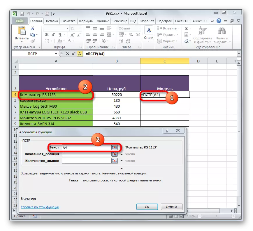
1. We produce the selection of the first cell of the column where the data will be displayed, and by the already familiar way, call the argument window of the PSTR function.

   In the "Text" field, as usual, specify the first cell of the column with the source data. Everything is no change here.



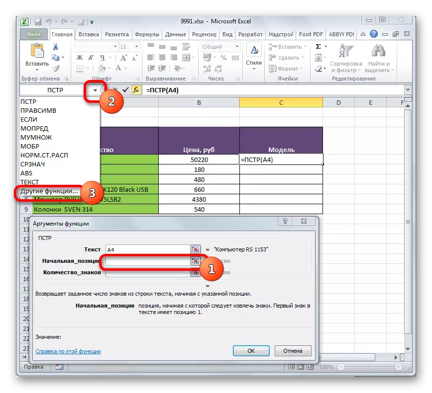
2. But the value of the "Starting Position" field will set the argument that generates a search function. As you can see, all data in the list combines the fact that before the model name there is a space. Therefore, the search operator will search for the first gap in the source range and report the number of this symbol of the PSTR function.

   In order to open the operator's arguments window, set the cursor in the "Starting position" field. Next, click on the icon in the form of a triangle directed by an angle down. This icon is located on the same horizontal level of the window, where the "Insert function" button is located and the formula string, but to the left of them. The list of recent operators applied. Since among them there is no name "Search", then click on the item "Other functions ...".



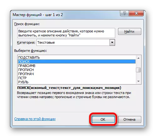
3. The Master of Function Wizard opens. In the category "Text" allocate the name "Search" and click on the "OK" button.



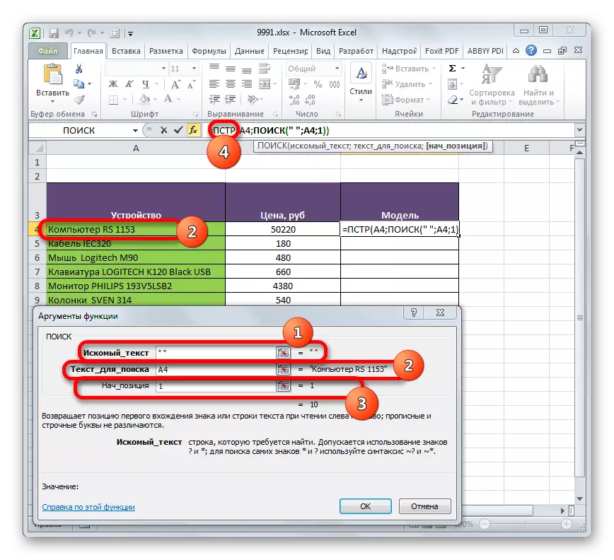
4. The operator's arguments window search starts. Since we are looking for a space, then in the field "The School Text" put the space, installing the cursor and pressing the appropriate key on the keyboard.

   In the "Text for Search" field, specify a link to the first cell of the source column. This link will be identical to the one that we previously indicated in the "Text" field in the Argument window of the PSTR operator.

   The argument of the field "Starting position" is not required to fill. In our case, it does not need to be filled or you can set the number "1". With any of these options, the search will be carried out from the beginning of the text.

   After the data is entered, do not rush to press the "OK" button, since the search function is nested. Just click on the name of the PSTR in the formula row.



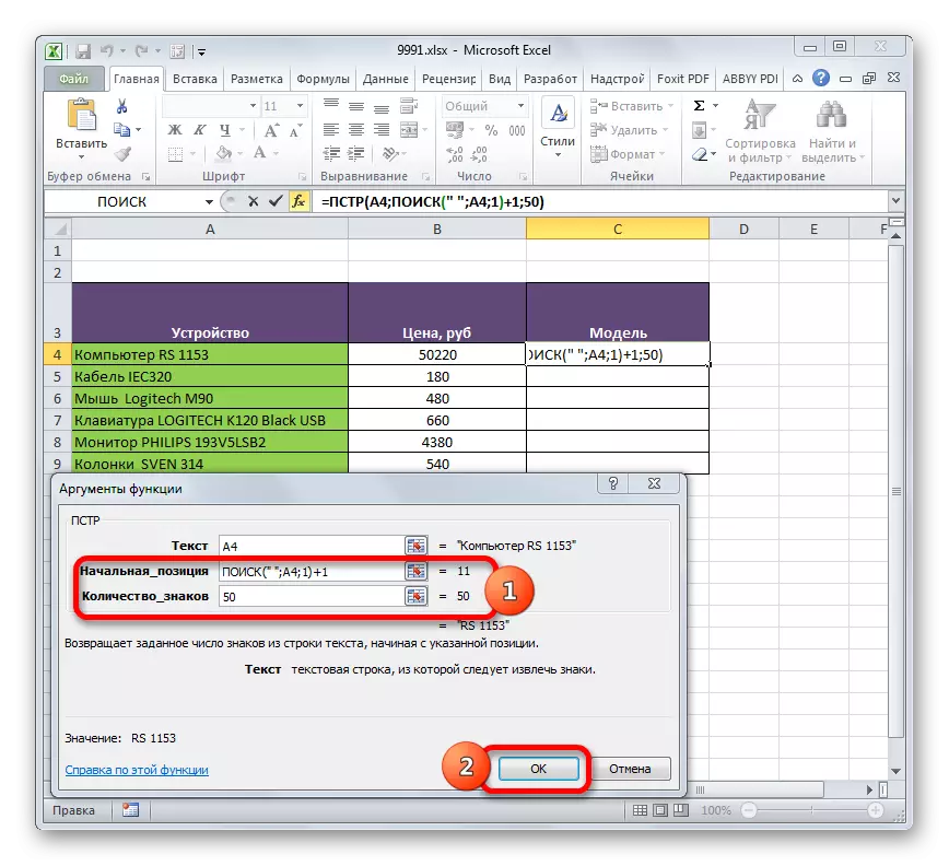
5. After completing the last specified action, we automatically return to the operator's arguments window of the PSTR. As you can see, the "Starting Position" field has already been filled with a search formula. But this formula points to the gap, and we need the next symbol after the space bar, from which the model name begins. Therefore, to existing data in the "Starting Position" field, we add the expression "+1" without quotes.

   In the "Number of Signs" field, as in the previous example, write any number that is greater than or equal to the number of characters in the longest expression of the source column. For example, we set the number "50". In our case, this is quite enough.

   After performing all these manipulations, press the "OK" button at the bottom of the window.



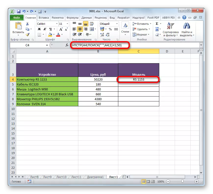
6. As we can see, after this, the name of the device model was displayed in a separate cell.



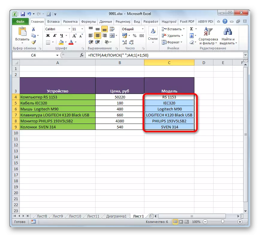
7. Now, using the filling wizard, as in the previous method, copy the formula on the cells, which are located below in this column.



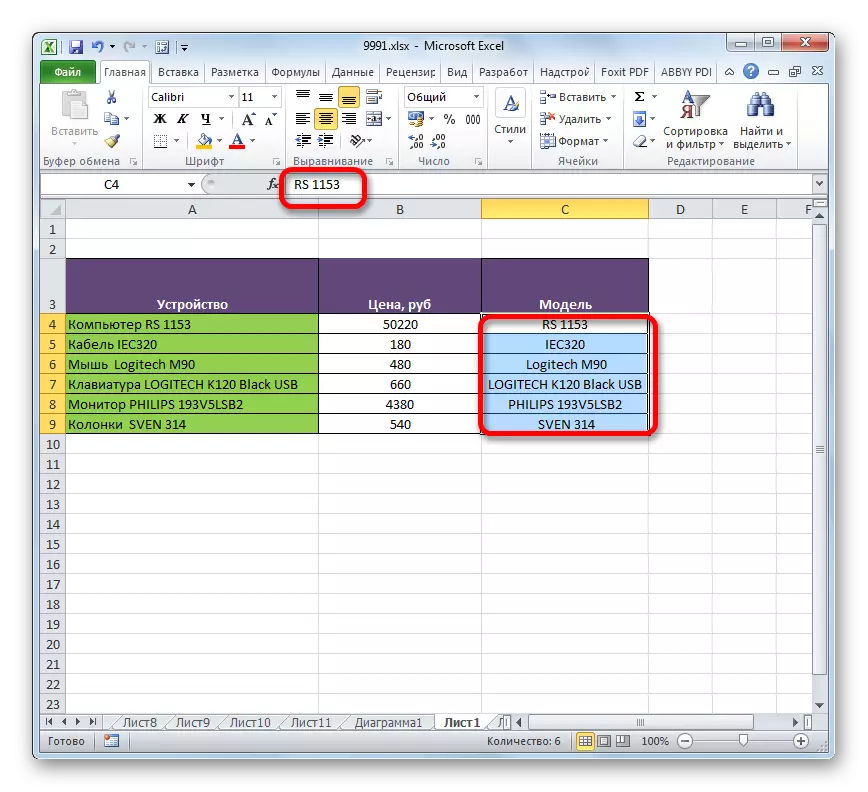
8. The names of all models of devices are displayed in the target cells. Now, if necessary, you can break the link in these elements with the source data column, as the previous time, applying consistently copying and inserting values. However, the specified action is not always mandatory.

The found function is used in combination with the formula of the Pastro, as the same principle as the search operator.

As you can see, the PSTR function is a very convenient tool for outputting the desired data into a predetermined cell. The fact that it is not so popular among users is explained by the fact that many users using Excel pay more attention to mathematical functions, not textual. When using this formula, combined with other operators, the functionality increases even more.