How to freeze the cell in Excel

Excel is dynamic tables, when working with which elements are shifted, addresses change, etc. But in some cases you need to fix a certain object or, as they say differently, to freeze so that it does not change its location. Let's figure out what options allow it to do.

Types of fixation

Immediately need to say that types of fixation in exile can be completely different. In general, they can be divided into three large groups:

1. Freezing addresses;
2. Fastening cells;
3. Protection of elements from editing.

When freezing the address, the link to the cell does not change when it is copying it, that is, it ceases to be relative. Consignment of cells allows you to see them constantly on the screen, no matter how far the user does not scroll down the sheet down or right. Protection of elements from editing blocks any data changes in the specified element. Let's consider in detail each of these options.

Method 1: Freeze Addresses

First, we will focus on fixing the cell addresses. To freeze it, from a relative reference, what is any address in Excel by default, you need to make an absolute link that does not change coordinates when copying. In order to do this, you need to install the address of the dollar sign ($) from each coordinate.

Setting the dollar sign is made by pressing the appropriate symbol on the keyboard. It is located on one key with a number "4", but to remove the screen you need to press the key in the English keyboard layout in the upper case (with the "SHIFT" key). There is a simpler and fast way. You should select the address of the element in a particular cell or in the row of functions and click on the F4 function key. When you first click, the dollar sign will appear at the address of the string and column, during the second click on this key it will remain only at the address of the line, during the third clicking - at the address of the column. Fourth Pressing the F4 key removes the dollar sign completely, and the next starts this procedure by a new circle.

Let's take a look at the address freezing on a specific example.

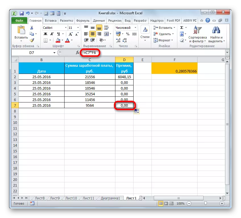
1. To begin with, copy the usual formula to other elements of the column. To do this, use the filling marker. Install the cursor to the lower right corner of the cell, the data from which you want to copy. At the same time, it is transformed into a cross, which carries the name of the filling marker. Push the left mouse button and pull this cross down to the end of the table.



2. After that, we allocate the lowest element of the table and look at the formula row, as the formula has changed during copying. As you can see, all coordinates that were in the very first element of the column, when copying shifted. As a result, the formula issues an incorrect result. This is due to the fact that the address of the second factor, in contrast to the first, should not be shifted for the correct calculation, that is, it needs to be made absolute or fixed.



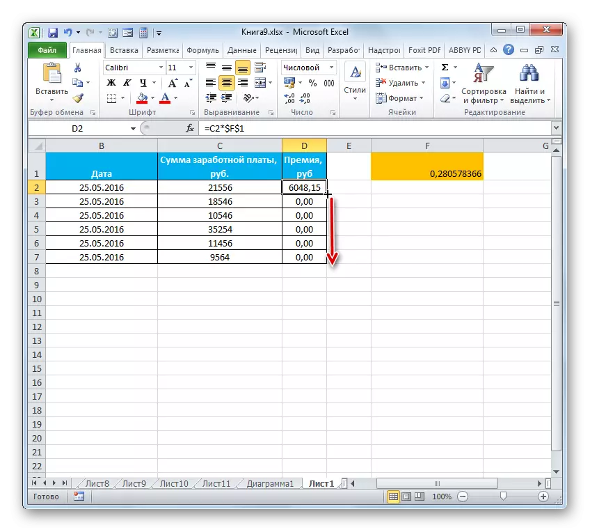
3. We return to the first element of the column and install the dollar sign near the coordinates of the second factor in one of those methods that we talked above. Now this link is frozen.



4. After that, using the filling marker, copy it to the table range located below.



5. Then we allocate the last element of the column. As we can observe through the formula string, the coordinates of the first factor are still shifted when copying, but the address in the second multiplier, which we made absolutely, does not change.



6. If you put the dollar sign only at the column coordinate, then in this case the address of the link column will be fixed, and the coordinates of the string are shifted when copying.



7. Conversely, if you set the dollar sign near the address of the line, then when copying it will not shift, unlike the address of the column.

This method produces freezing coordinates of cells.

Lesson: Absolute Addressing in Excel

Method 2: Fixing cells

Now we learn how to fix the cells so that they constantly remain on the screen where the user would not go within the leaf boundaries. At the same time, it should be noted that the individual element cannot be fastened, but you can fix the area in which it is located.

If the desired cell is located in the upper line of the sheet or in the leftmost column, then the fixation is elementary simply.

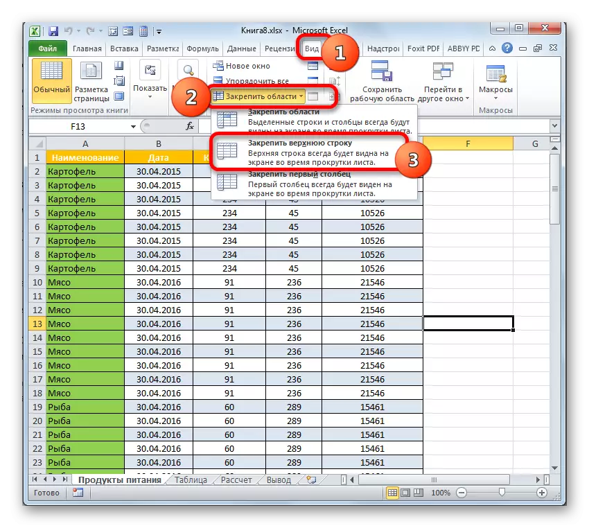
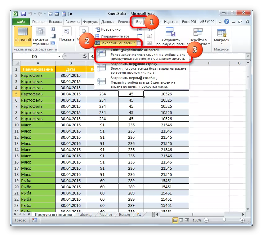
1. To secure the string, perform the following actions. Go to the "View" tab and clay on the "Fasten Area" button, which is located in the window of the "Window" toolbar. A list of different assignment options opens. Choose the name "Secure the upper line".



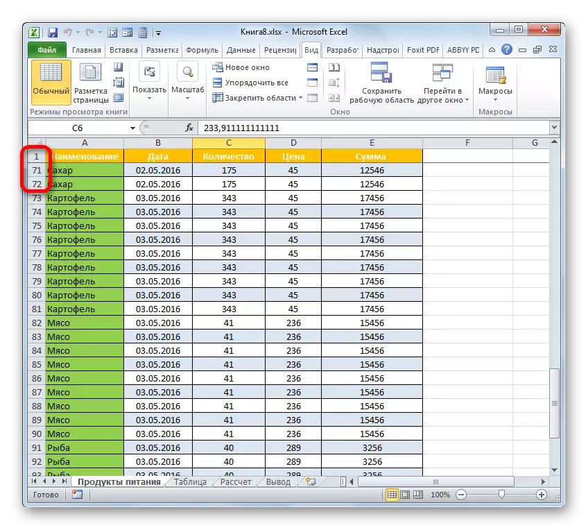
2. Now even if you descend to the bottom of the sheet, the first line, which means that the item you need, located in it, will still be at the very top of the window.

Similarly, you can freeze the extreme left column.

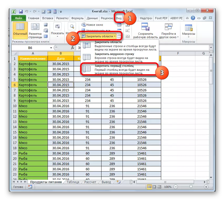
1. Go to the "View" tab and click on the "Fasten Area" button. This time I choose the option "Secure the first column".



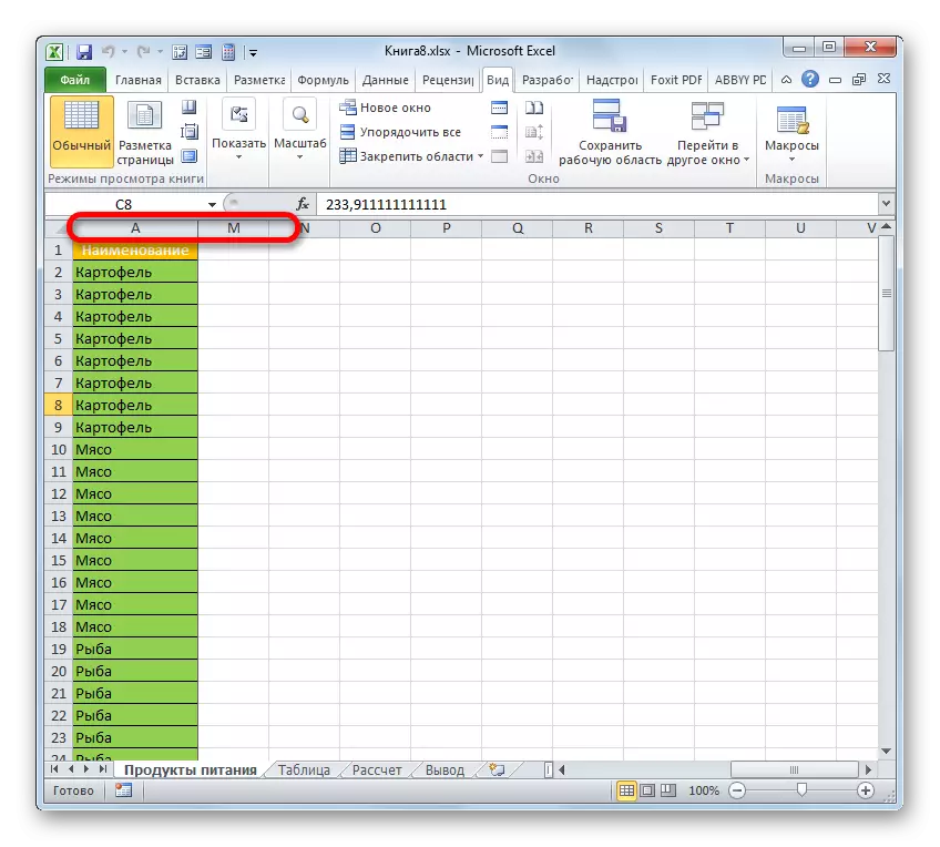
2. As you can see, the most extreme left column is now fixed.

Approximately the same way you can consolidate not only the first column and string, but in general, the entire area is left and above from the selected item.

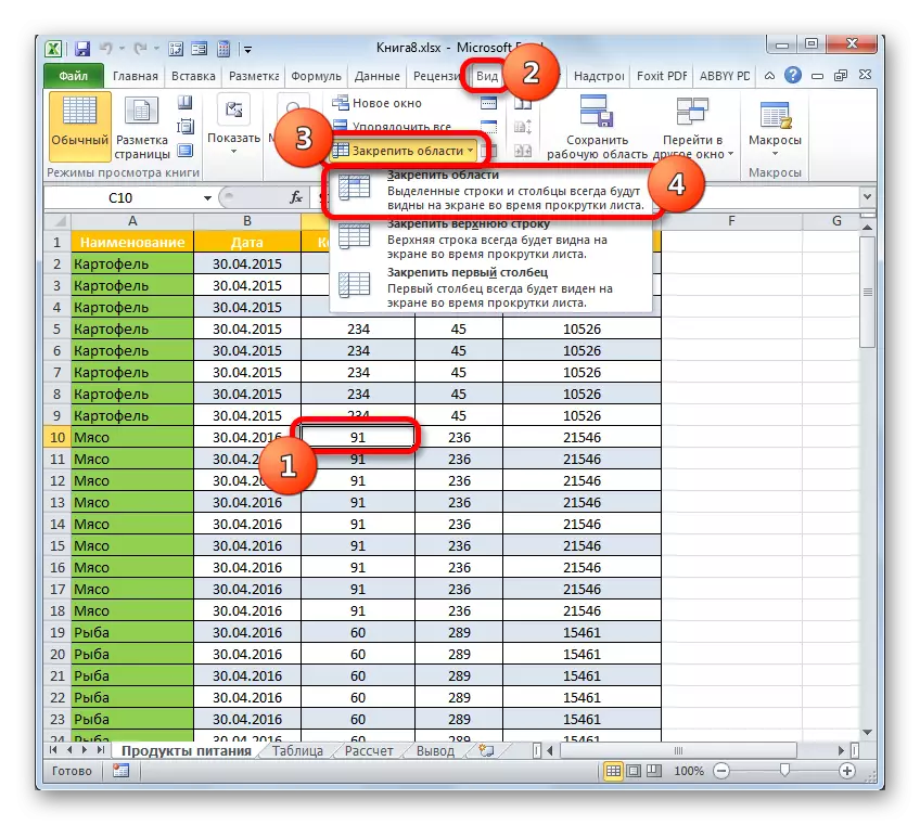
1. The execution algorithm for this task is slightly different from the previous two. First of all, it is necessary to highlight the leaf element, the area from above and the left of which will be fixed. After that, go to the "View" tab and click on a familiar icon "Fasten the Area". In the menu that opens, select the item with exactly the same name.



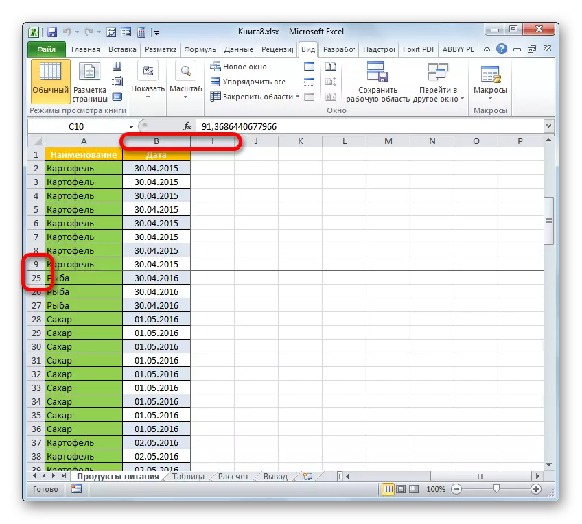
2. After this action, the entire area located on the left and above the dedicated element will be fixed on the sheet.

If desired, remove the freezing made in this way, quite simple. The execution algorithm is the same in all cases that it would be the user who would not secure: a string, column or area. We move to the "View" tab, click on the "Fix the Area" icon and in the list that opens, select the option to "remove the consolidation of regions". After that, all fixed ranges of the current sheet will be dropped.

Lesson: How to fix the area in Excel

Method 3: Editing Protection

Finally, you can protect the cell from editing by blocking the ability to make changes to users. Thus, all the data that is in it will be actually frozen.

If your table is not dynamic and does not provide for the introduction of any changes in it, you can protect not only specific cells, but also the entire sheet as a whole. It is even much easier.

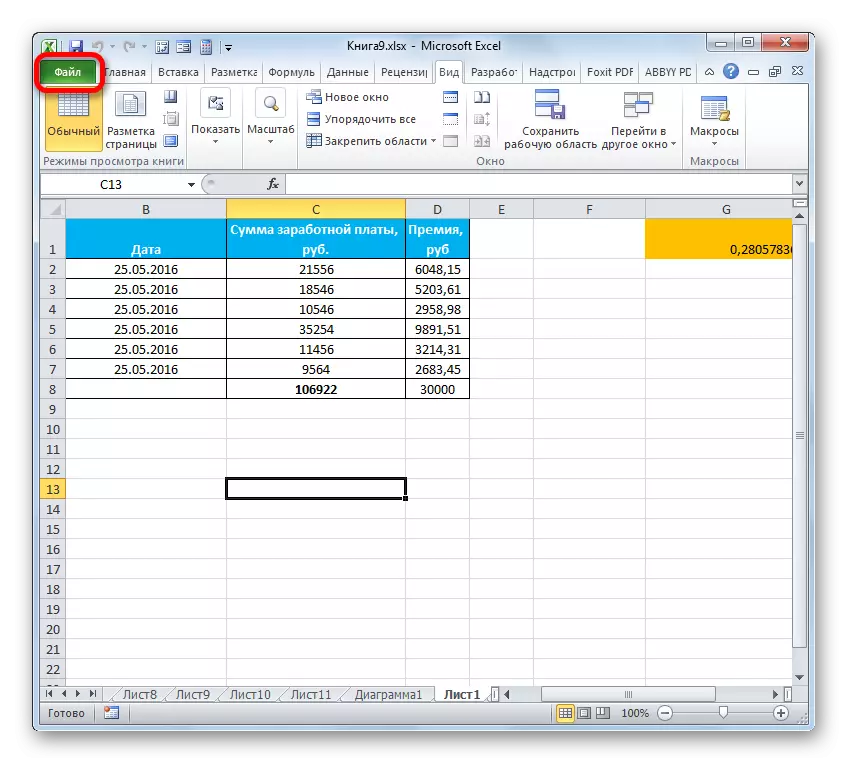
1. Move into the "File" tab.



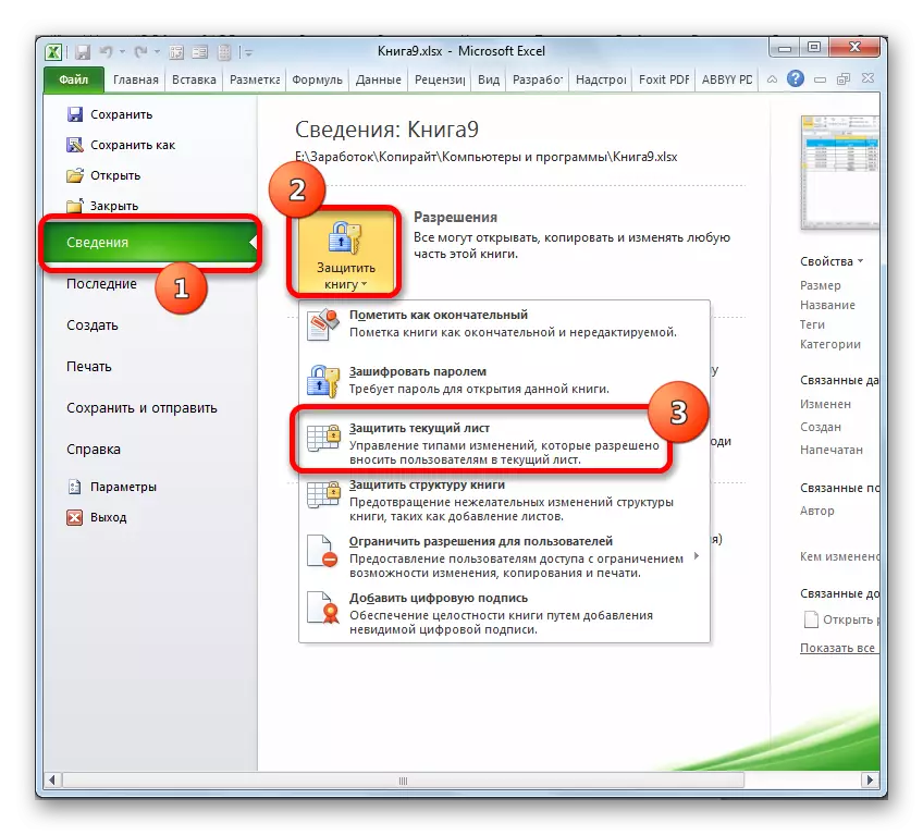
2. In the window that opens in the left vertical menu, go to the "Details" section. In the central part of the window, clay on the inscription "Protect the book". In the list of security actions that opens, choose the "Protect Current Sheet" option.



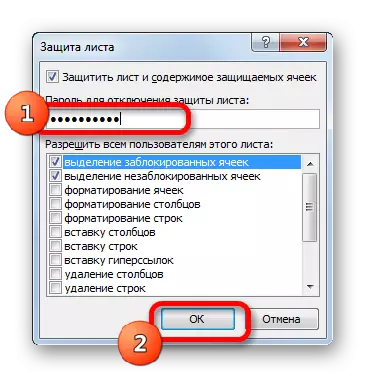
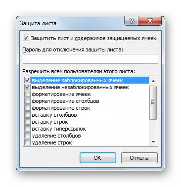
3. A small window is launched, which is called "Sheet Protection". First of all, in it in a special field you need to enter an arbitrary password, which will be needed by the user if it wishes to disable the protection in the future to edit the document. In addition, at will, you can install or remove a number of additional restrictions, installing or removing flags near the respective items in the list presented in this window. But in most cases, the default settings are quite consistent with the task, so that you can simply click on the "OK" button after entering the password.



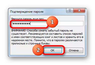
4. After that, another window starts, in which the password entered earlier should be repeated. This is done to ensure that the user has been confident that it introduced exactly the password that I remembered and wrote in the appropriate layout of the keyboard and the register, otherwise it myself can lose access to editing the document. After re-entering the password, press the "OK" button.



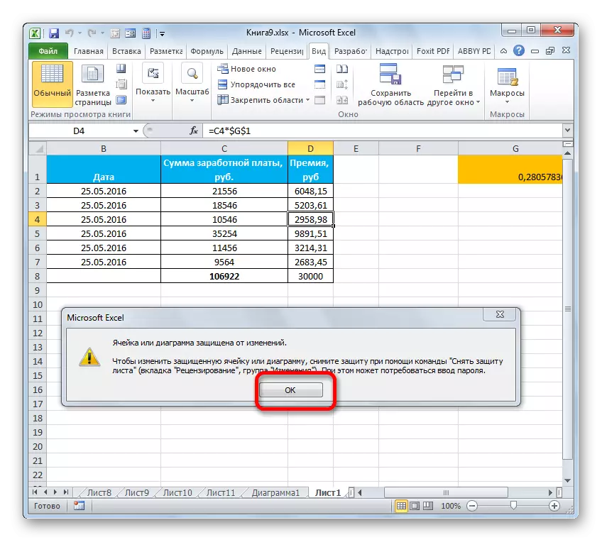
5. Now when trying to edit any sheet item, this action will be blocked. The information window will open, reporting on the impossibility of changing data on a protected sheet.

There is another way to block any changes in the elements on the sheet.

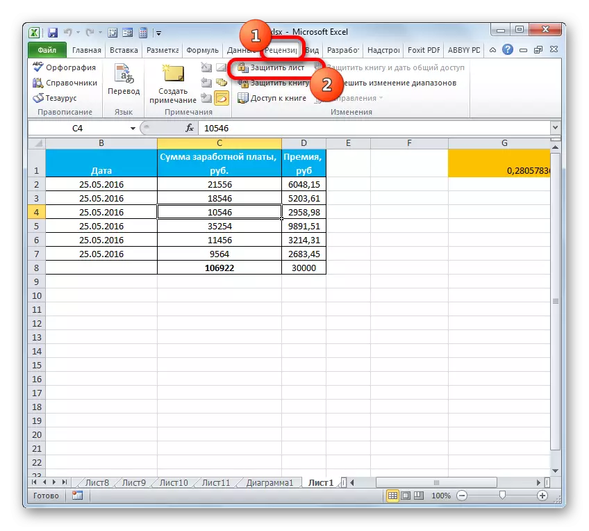
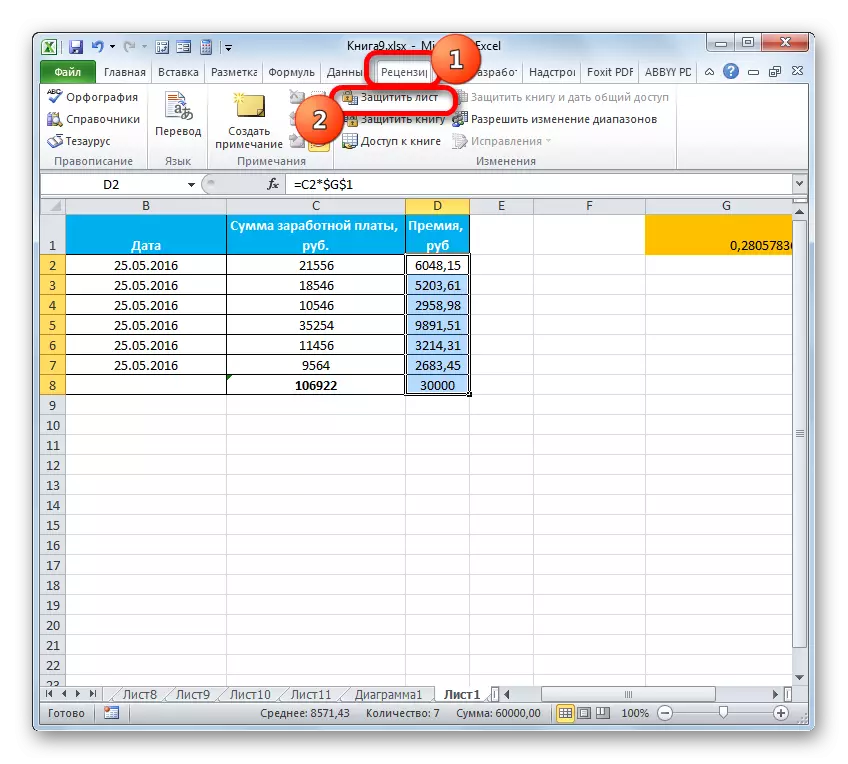
1. Go to the "Review" window and clay on the "Protect Leaf" icon, which is located on the tape in the "Change" tool block.



2. Opened already familiar to us window protection window. All further action perform in the same way as described in the previous version.

But what to do if you need to freeze only one or more cells, and in others it is assumed, as before, to freely make data? There is a way out of this position, but its solution is somewhat more complicated than the previous task.

In all cells of the default document in the properties, the protection is shown, when the sheet lock is activated in general, the options mentioned above. We will need to remove the protection parameter in the properties of absolutely all sheet elements, and then set it again only in those elements that we wish to freeze from changes.

1. Click on a rectangle, which is located on the junction of horizontal and vertical coordinate panels. Also, if the cursor is in any area of ​​the sheet outside the table, press the combination of hot keys on the Ctrl + A keyboard. The effect will be the same - all elements on the sheet are highlighted.



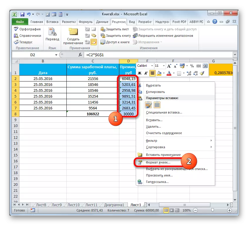
2. Then we clas on the highlight zone by right-click. In the activated context menu, select the "Cell Format ...". Also, instead, you can use the Ctrl + 1 key combination set.



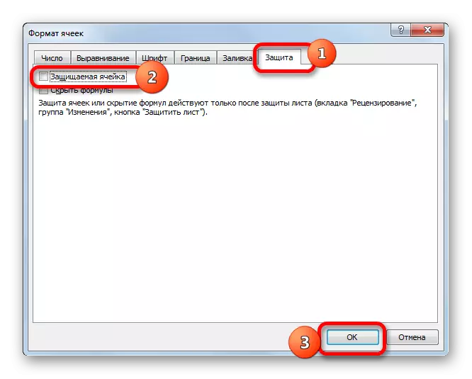
3. The "Cell Format" window is activated. Immediately transition to the "Protection" tab. It should be removed the checkbox near the "Protected Cell" parameter. Click on the "OK" button.



4. Next, we return to the sheet and allocate the element or group in which we are going to freeze the data. We click right-click on the dedicated fragment and in the context menu, go to the name "Cell format ...".



5. After opening the formatting window, once again go to the "Protection" tab and set the checkbox near the "Protected Cell" item. Now you can click on the "OK" button.



6. After that, we set the sheet protection by any of those two ways that were previously described.

After executing all the procedures described in detail us above, only those cells on which we re-installed protection through the properties of the format will be blocked from changes. In all other elements of the sheet, as before, you can freely contribute any data.

Lesson: how to protect the cell from changes to Excel

As you can see, there are three ways to freeze the cells. But it is important to note that it differs in each of them not only the technology of performing this procedure, but also the essence of the frost itself. So, in one case, only the address of the leaf element is recorded, in the second - the area is fixed on the screen, and in the third - the protection of data changes in the cells is set. Therefore, it is very important to understand before performing the procedure, what exactly are you going to block and why do you do it.