How to combine cells in Excel

Quite often, when working with tables in the Microsoft Excel program, the situation occurs when you need to combine several cells. The task is not too complicated if these cells do not contain information. But what to do if information has already been made in them? Will it be destroyed? Let's figure it out how to combine cells, including without losing their contents, in Microsoft Excel.

Combining cells in Excel

Consider the association in all methods in which cells will accommodate data. If two adjacent positions for future mergers have different information, they can be saved in both cases - for this, the office package provides special functions discussed below. The combination may be needed not only to make data from two cells into one, but also, for example, in order to create a hat for several columns.

Method 1: Simple Association

The easiest way to combine multiple cells is the use of the provided button in the menu.

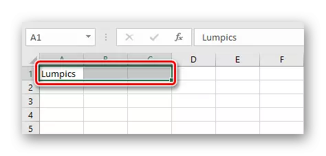
1. Sequentially select the left mouse button to merge. It can be rows, columns or alignment options. In the considered method, we use the row merging.



2. Go to the "Home" tab.



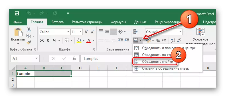
3. Find and click on the arrow of the context menu of the merger, where there are several possible options, among which choose the easiest of them - the "Combine cells" string.



4. In this case, the cells are combined, and all the data that will fit into the combined cell will remain in the same place.



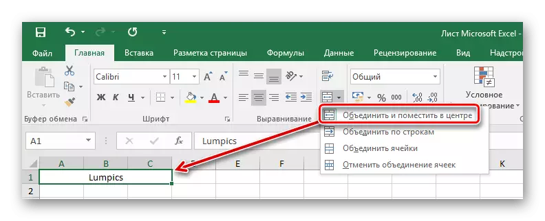
5. To format text after combining the center, you must select the item "Combining with alignment in the center". After actions made, the contents can be aligned in your own way using the appropriate tools.



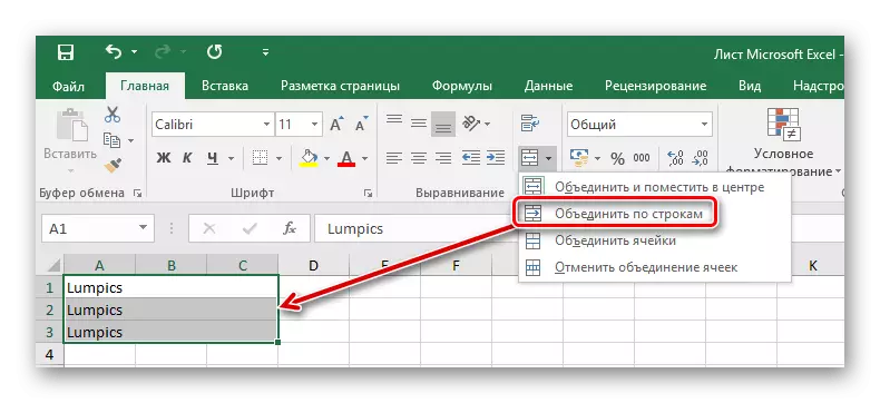
6. In order not to combine a large number of lines separately, use the "Row Association" function.

Method 2: Change Cell Properties

It is possible to combine cells through the context menu. The result obtained from this method is not different from the first, but someone can be more convenient to use.

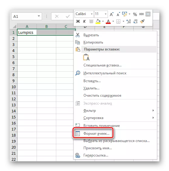
1. Highlight the cursor to the cells, which should be merged, click on it right-click, and in the context menu that appears, select "Cell format".



2. In the cell format window that opens, go to the Alignment tab. We celebrate the check box "Association of Cells". Immediately, other parameters can be installed: the direction and orientation of the text, the leveling horizontally and vertical, the width of the width, the transfer by words. When all settings are made, click on the "OK" button.



3. As you can see, the association of cells occurred.

Method 3: Union without loss

What to do if there are data in several of the combined cells, because when you merge all values ​​other than the top top will be lost? In this case, information is necessary from one cell to consistently add to the one that is in the second cell, and transfer them to a completely new position. With this, a special symbol of "&" (called "ampersant") or the formula "Capture (eng. Concat)" can cope with this.

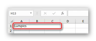
Let's start with a simpler option. All you need to do is specify the path to the combined cells in the new cell, and insert a special symbol between them. Let's connect three cells at once in one, thus creating a text string.

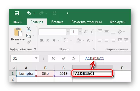
1. Select a cell in which you wish to see the result of the union. In it, write the sign of the equality "=" and sequentially select specific positions or a whole range of data for merge. Between each cell or range should be a sign of ampersant "&". In the specified example, we combine the cells "A1", "B1", "C1" in one - "D1". After entering the function, click "Enter".



2. Due to the previous action in the cell with the formula, all three positions were merged into one.



3. In order for the text at the end, you can add spaces between the cells. In any formula, to add an incidence between data, you must enter a space in brackets. Therefore, insert it between "A1", "B1" and "C1" in this way: "= A1 &" "& B1 &" "& C1".



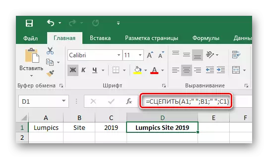
4. The formula suggests about the same principle - the specified cells or ranges will be merged into the place where you prescribe the function "= Capture ()". Considering an example of ampersant, replacing it to the mentioned function: "= Catch (A1;" "; B1;" "; C1)." Please note that spaces are immediately added for convenience. In the formula, the space is taken into account as a separate position, that is, we add a space to the A1 cell, then the B1 cell and so on.



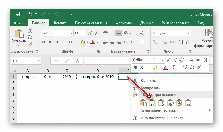
5. If you need to get rid of the source data that were used to merge, leaving only the result, you can copy the processed information as a value and remove the extra columns. To do this, copy the finished value in the "D1" cell combination of the "Ctrl + C" keys, right-click on the free cell and select "Values".



6. As a result - a clean result without a formula in the cell. Now you can delete previous information convenient for you.

If the usual cell combining in the Microsoft Excel program is quite simple, then with the association of cells without losses will have to be tinted. Nevertheless, this is also done by the task for this kind of program. The use of features and special characters will save a lot of time on the processing of a large amount of information.