How to make a chart in exile

Microsoft Excel allows not only convenient to work with numeric data, but also provides tools for building diagrams based on the parameters entered. Their visual display can be completely different and depends on the user solutions. Let's figure out how to draw different types of diagrams using this program.

Building Chart in Excel

Because through Excel you can flexibly process numerical data and other information, the tool for constructing diagrams here also works in different directions. In this editor, there are both standard types of diagrams based on standard data and the ability to create an object for a demonstration of interest ratios or even a clearly reflecting Pareto law. Next, we will talk about different methods of creating these objects.

Option 1: Build chart on the table

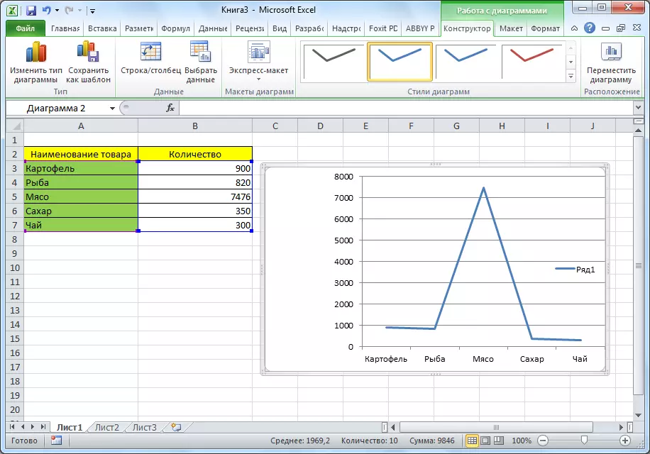
The construction of various types of diagrams is practically no different, only at a certain stage you need to select the appropriate type of visualization.

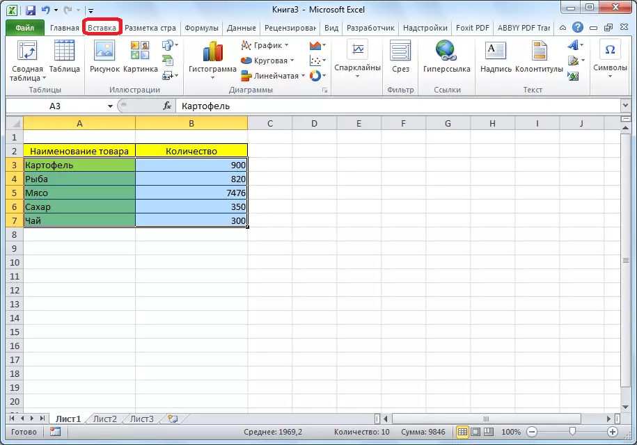
1. Before you begin to create any chart, it is necessary to build a table with data on the basis of which it will be built. Then go to the "Insert" tab and allocate the area of ​​the table, which will be expressed in the diagram.



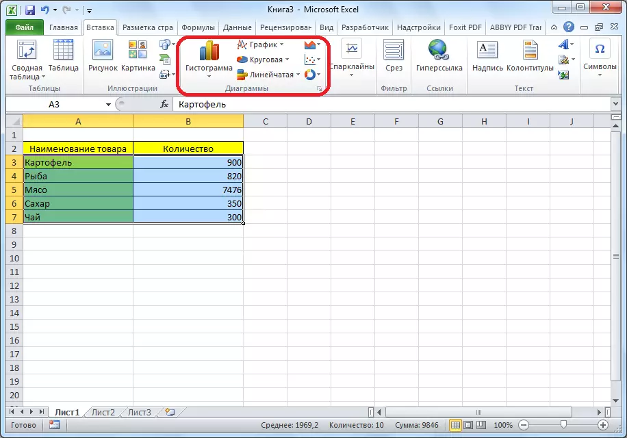
2. On the tape at the Insert Deposte, we choose one of the six main types:
   • Bar graph;
   • Schedule;
   • Circular;
   • Linear;
   • With regions;
   • Point.



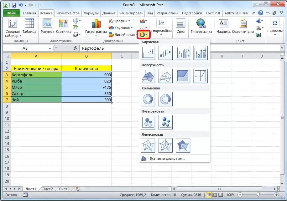
3. In addition, by clicking on the "Other" button, you can stop at one of the less common types: stock, surface, ring, bubble, petal.



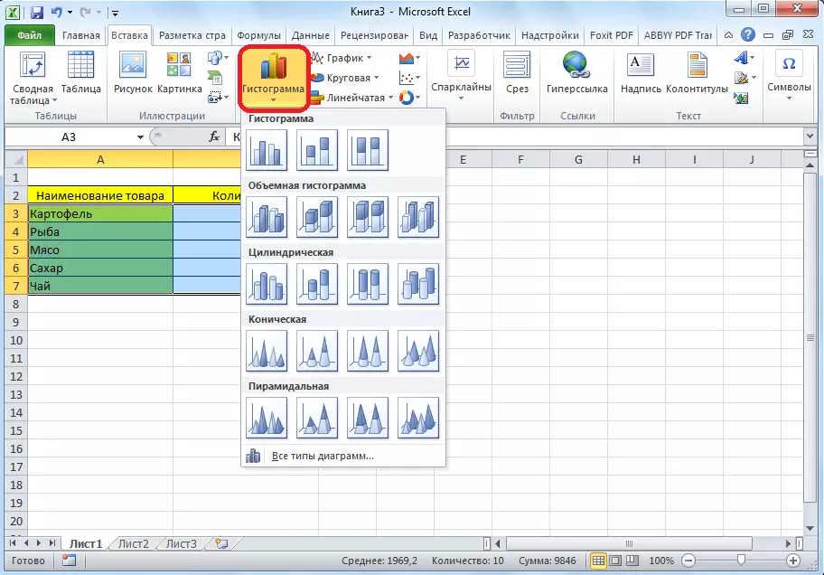
4. After that, clicking on any of the types of charts, the ability to choose a specific subspecies. For example, for a histogram or bar diagram, such subspecies will be the following elements: the usual histogram, bulk, cylindrical, conical, pyramidal.



5. After selecting a specific subspecies, a diagram is automatically formed. For example, the usual histogram will look like shown in the screenshot below:



6. The chart in the form of a graph will be as follows:



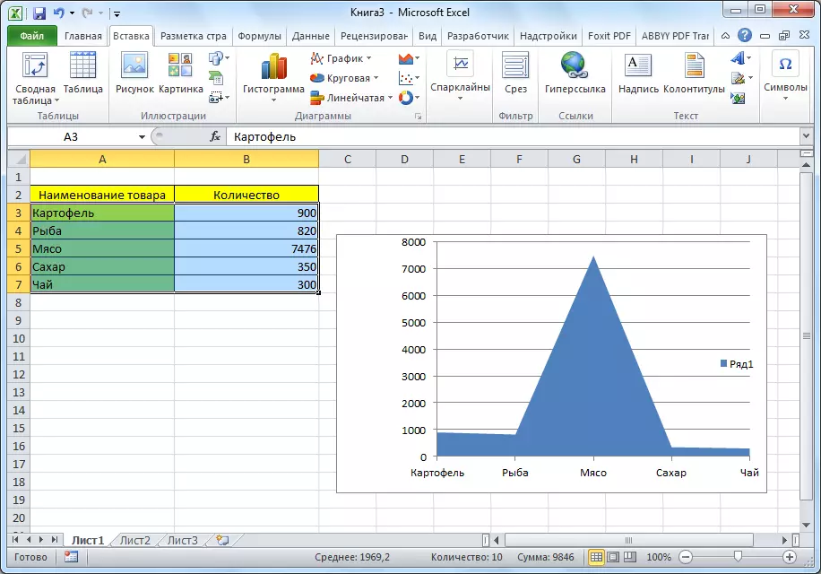
7. Option with regions will take this kind:

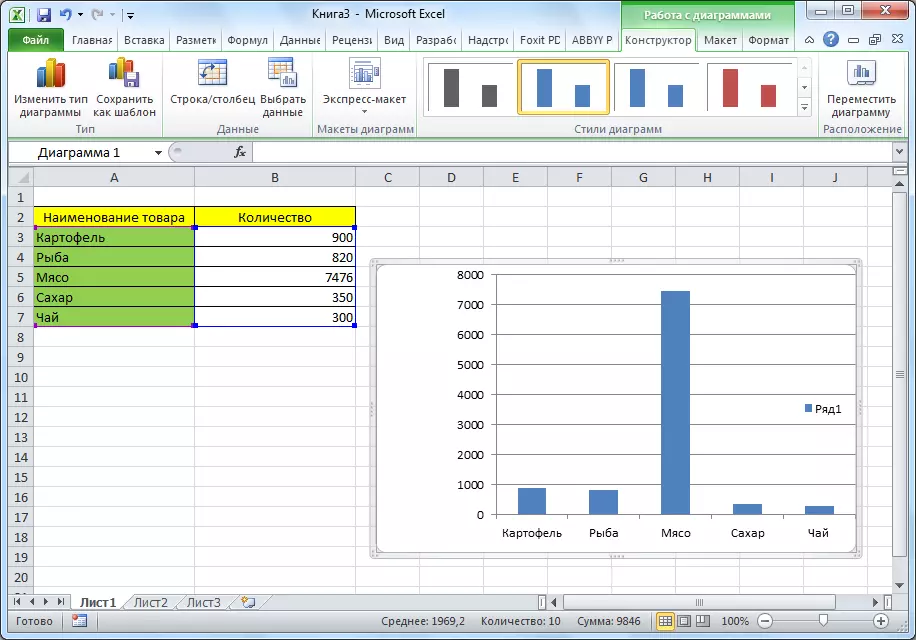
Working with diagrams

After the object was created, additional instruments for editing and change becomes available in the new tab "Working with Charts".

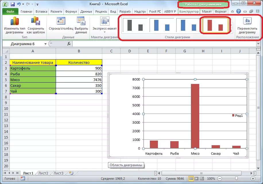
1. Available Change type, style and many other parameters.



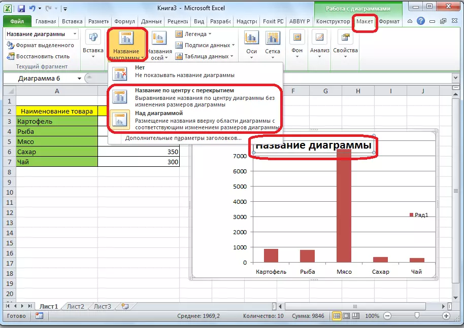
2. The "Work with Charts" tab has three additional subfolded tabs: "Designer", "layout" and "format", using which, you can adjust its mapping as it will be necessary. For example, to name a diagram, open the tab "Layout" and select one of the names of the name: in the center or from above.



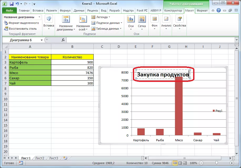
3. After it was done, the standard inscription "Diagram name" appears. We change it on any inscription suitable in the context of this table.



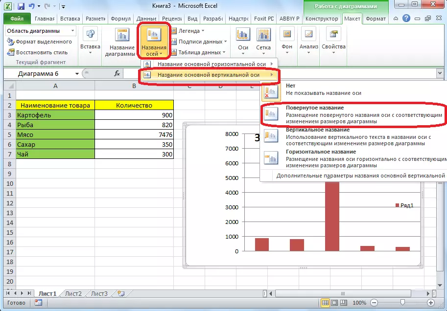
4. The name of the diagram axes is signed by exactly the same principle, but for this you need to press the "axis names" button.

Option 2: Display chart in percent

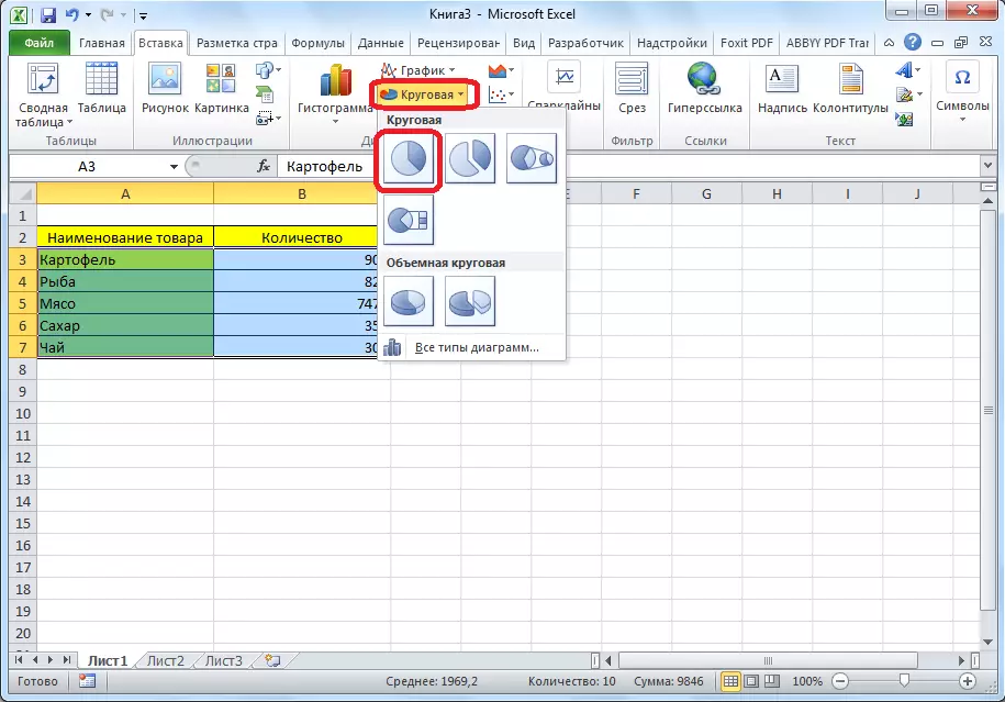
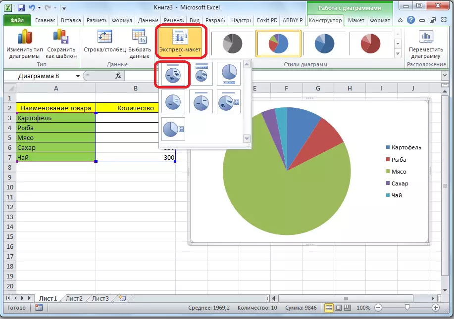
To display the percentage ratio of various indicators, it is best to build a circular diagram.

1. Similarly, how we were told, we build a table, and then select the data range. Next, go to the "Insert" tab, specify a circular diagram on the tape and in the Click list that appears on any type.



2. The program independently translates us into one of the tabs to work with this object - "Designer". Choose among the layouts in the ribbon of any, in which there is a percent symbol.



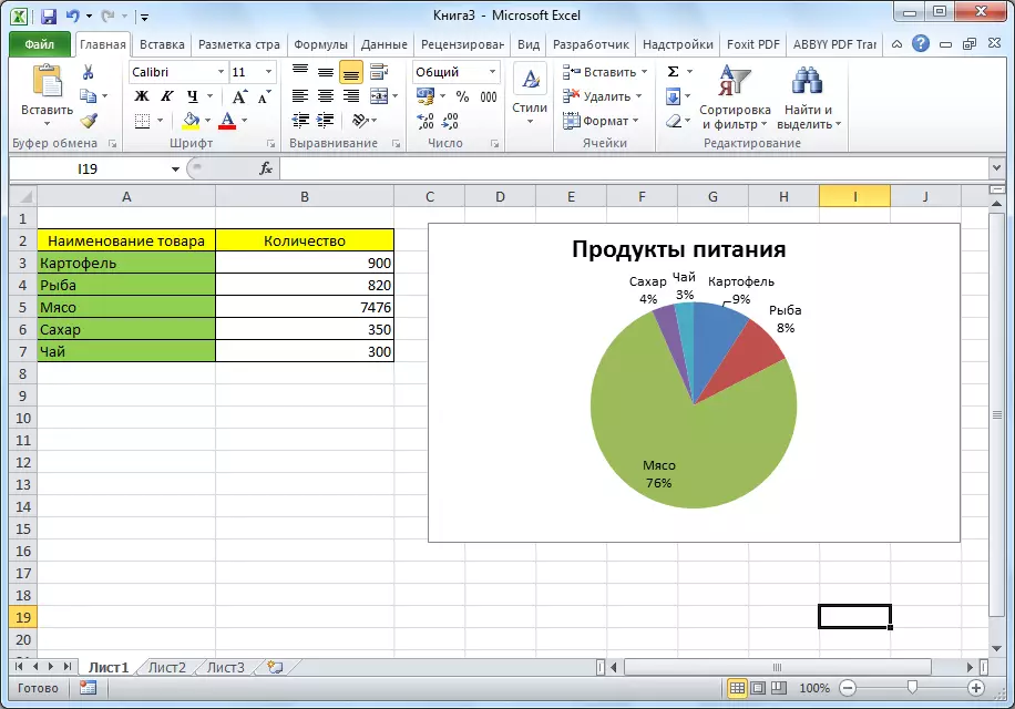
3. Circular diagram with data display in percent is ready.

Option 3: Build Chart Pareto

According to Wilfredo Pareto theory, 20% of the most effective actions bring 80% of the general result. Accordingly, the remaining 80% of the total aggregate of actions that are ineffective, only 20% of the result brought. Building Chart Pareto is just designed to calculate the most effective actions that give the maximum return. Make it using Microsoft Excel.

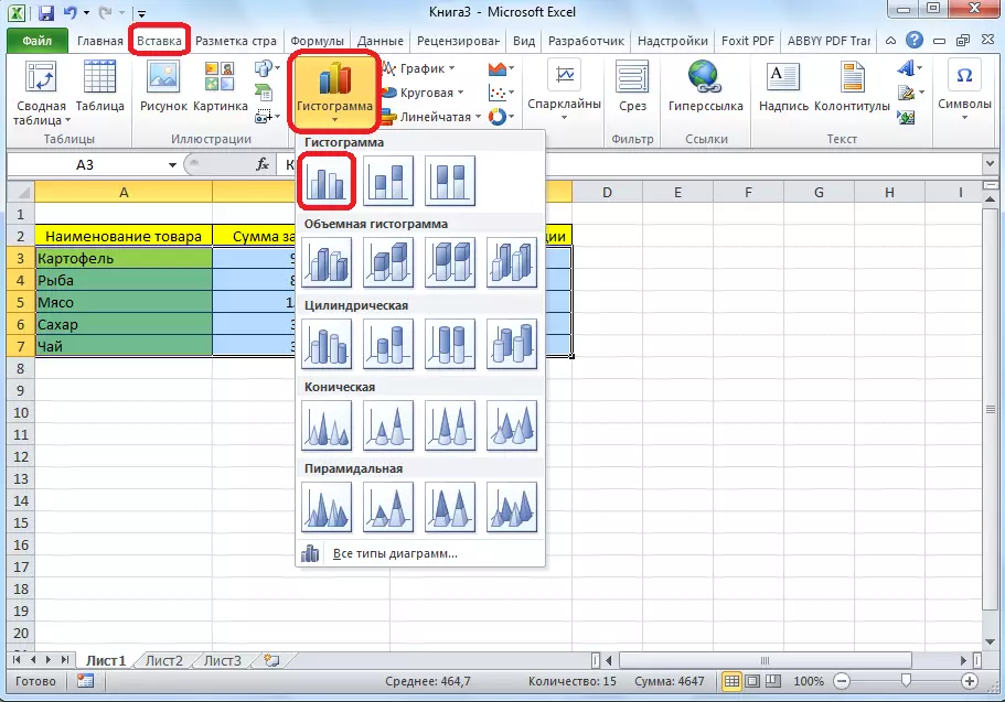
1. It is most convenient to build this object in the form of a histogram, which we have already spoken above.
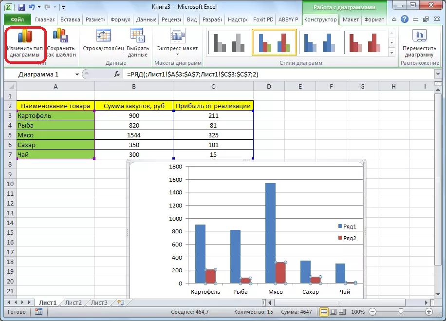
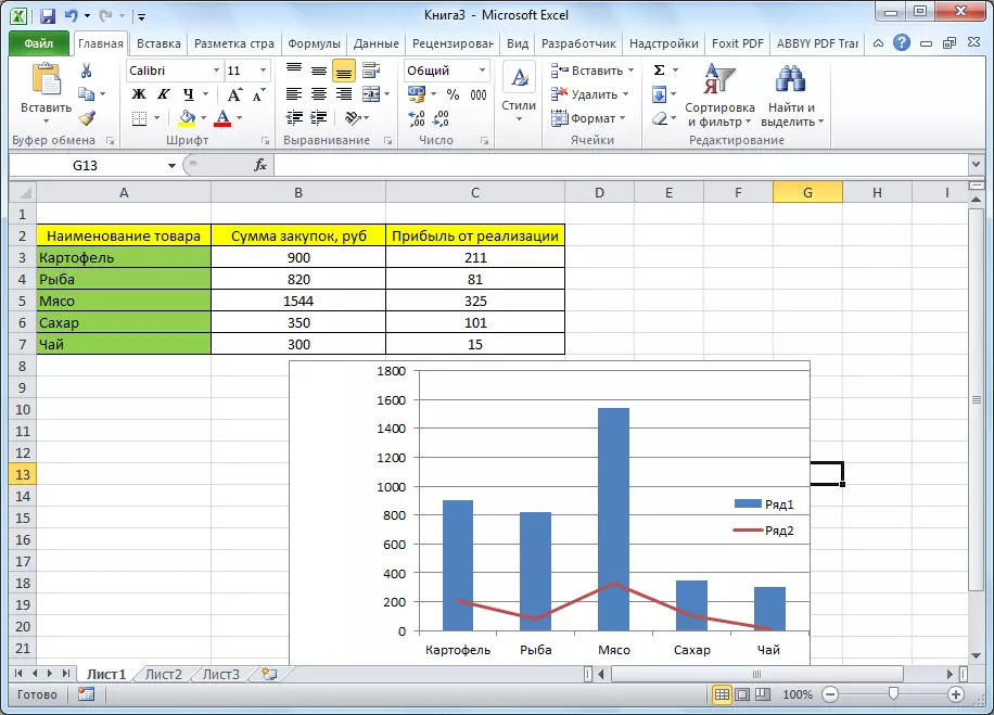
2. Let us give an example: the table contains a list of food. In one column, the procurement value of the entire volume of the specific type of products on the wholesale warehouse was inscribed, and in the second - profit from its implementation. We have to determine which goods give the greatest "return" when selling.

   First of all, we build a typical histogram: we go to the "Insert" tab, we allocate the entire area of ​​the table values, click the "Histogram" button and select the desired type.



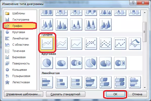
3. As you can see, a chart with two types of columns was formed as a result: blue and red. Now we should convert red columns to the schedule - select these columns with the cursor and on the "Designer" tab by clicking on the "Change Type of Chart" button.



4. A window change window opens. Go to the "schedule" section and specify the type suitable for our purposes.



5. So, the Pareto diagram is built. Now you can edit its elements (name of the object and axes, styles, etc.) just as described on the example of a columnar chart.

As you can see, Excel presents many functions for building and editing various types of diagrams - the user remains to decide which type and format is necessary for visual perception.