Creating Summary Tables in Excel

Excel's summary tables provide users with users in one place to group significant amounts of information contained in bulky tables, as well as compile comprehensive reports. Their values ​​are updated automatically when changing the value of any associated table. Let's find out how to create such an object in Microsoft Excel.

Creating a pivot table in Excel

Since, depending on the result, which the user wants to receive, the consolidated table can be both simple and difficult to compose, we will look at two ways to create it: manually and using the built-in tool program. Additionally, we will tell you how such objects are configured.

Option 1: Normal Summary Table

We will consider the process of creating on the example of Microsoft Excel 2010, but the algorithm is applicable for other modern versions of this application.

1. As a basis, we take the payroll payroll table to employees of the enterprise. It contains the names of workers, the floor, category, date and amount of payment. That is, each episode of payments to a separate employee corresponds to a separate line. We have to group chaoticly located data in this table in one pivot table, and the information will be taken only for the third quarter of 2016. Let's see how to do this on a specific example.
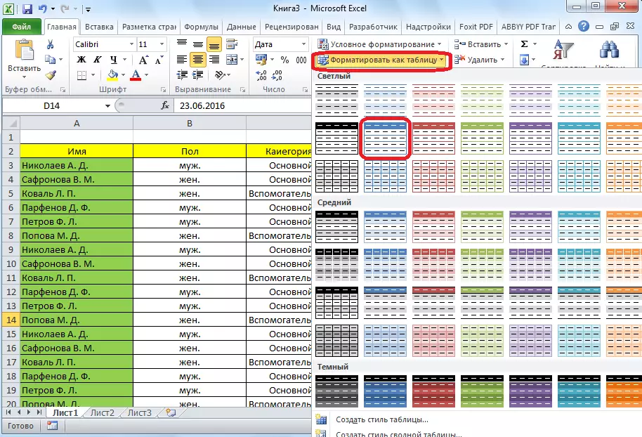
2. First of all, we transform the source table into dynamic. It is necessary in order to be automatically tightened to the consolidated table when adding lines and other data. We carry the cursor to any cell, then in the "Styles" block located on the tape, click on the "Format as a table" button and choose any like-like table style.



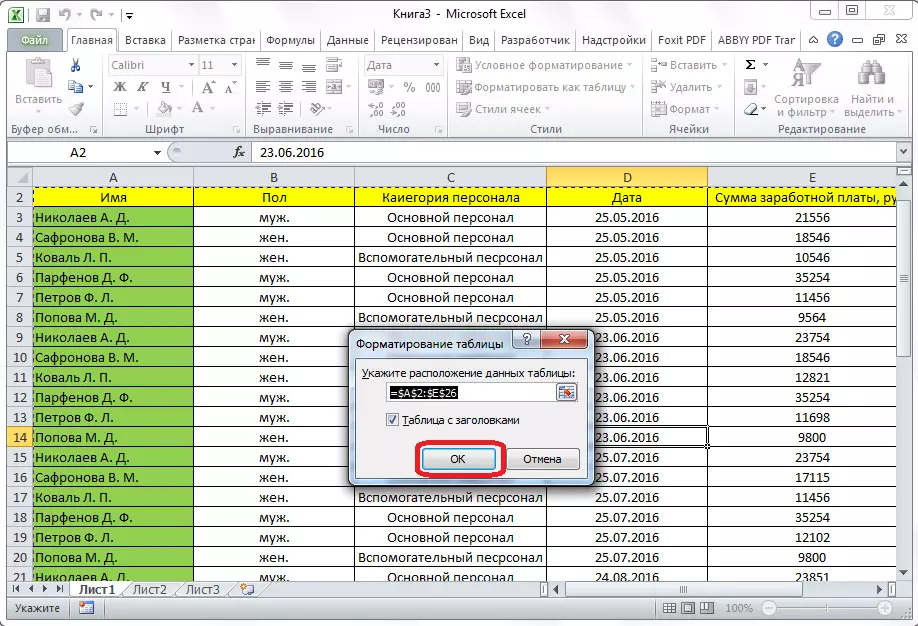
3. The dialog box opens, which we offer to specify the coordinates of the table location. However, by default, the coordinates that the program offers, and so cover the entire table. So we can only agree and click on "OK". But users need to know that if desired, they can change these parameters here.



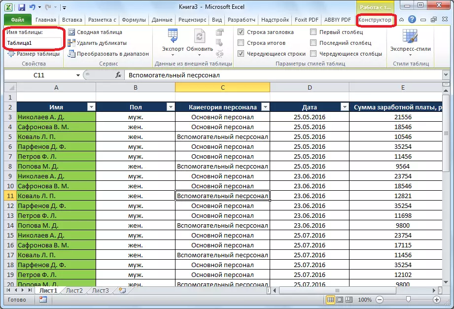
4. The table turns into a dynamic and automatically stretching. She also gets a name that, if desired, the user can change to any convenient. You can view or change the name on the Designer tab.



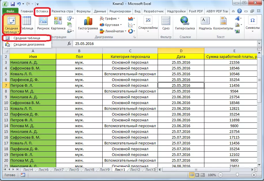
5. To directly start creating, choose the "Insert" tab. Here we click on the first button in the ribbon, which is called the "Summary Table". A menu will open, where you should choose that we are going to create: a table or chart. At the end, click "Summary Table".



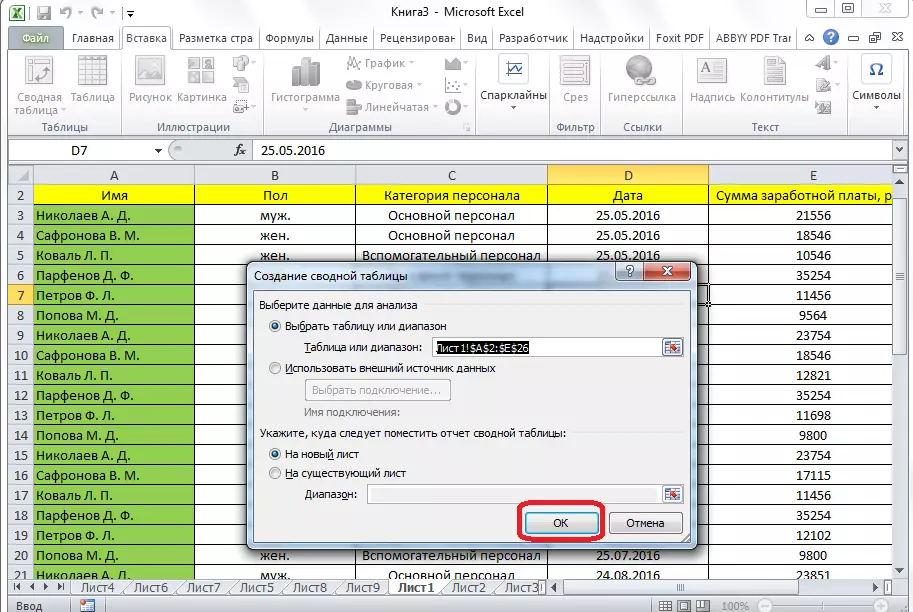
6. In a new window, we need to select a range or table name. As you can see, the program itself pulled the name of our table, so it's not necessary to do anything else. At the bottom of the dialog box, you can select a place where a summary table will be created: on a new sheet (default) or on the same one. Of course, in most cases, it is more convenient to keep it on a separate sheet.



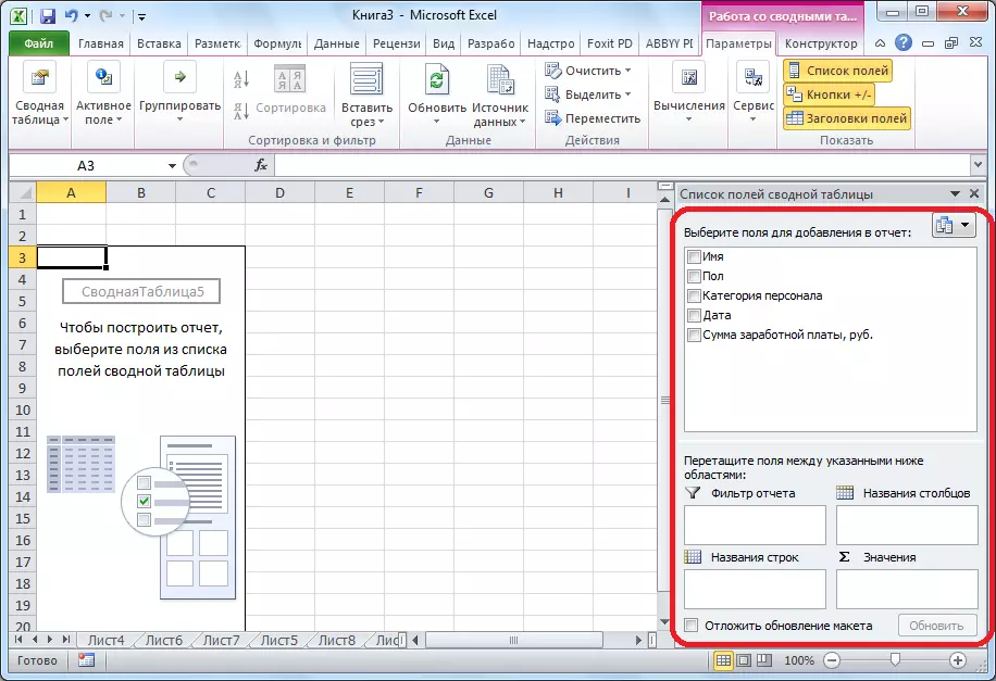
7. After that, on a new sheet, the form of creating a pivot table will open.
8. The right part of the window is a list of fields, and below four areas: string names, column names, values, report filter. Just dragging the tables of the table in the appropriate areas of the area you need. There is no clearly established rule, which fields should be moved, because it all depends on the original source table and on specific tasks that may vary.



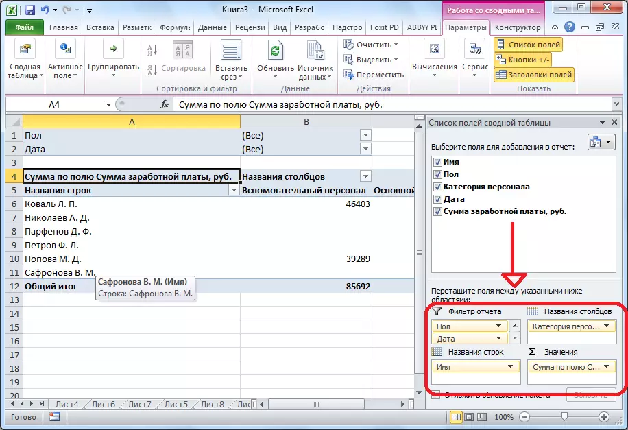
9. In a concrete case, we moved the fields "Paul" and "Date" to the Filter of the Report Filter, "Personnel Category" - in the "Column Names", "Name" - in the "Line name", "wage amount" - in "Values " It should be noted that all arithmetic calculations of data, taut from another table, are possible only in the last area. While we have done such manipulations with the transfer of fields in the area, the table itself on the left side of the window changes, respectively.



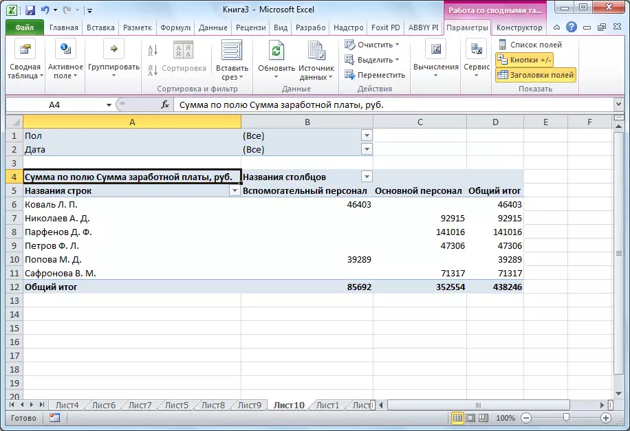
10. It turned out such a pivot table. The filters on the floor and date are displayed above it.

Option 2: Master of Summary Tables

You can create a summary table by applying the "Summary Wizard" tool, but for this immediately need to withdraw it to the "Quick Access Panel".

1. Go to the "File" menu and click on "Parameters".



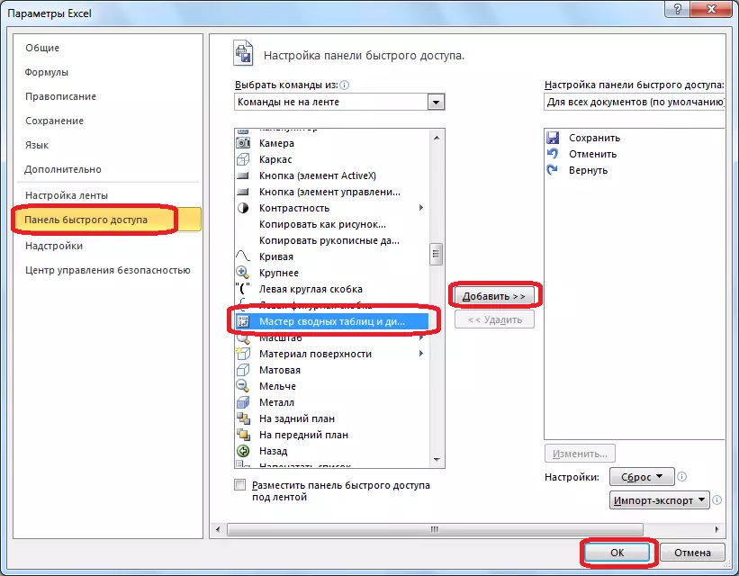
2. We go to the "Quick Access Panel" section and select commands from the commands on the tape. In the list of items are looking for "Master of Summary Tables and Charts". We highlight it, press the "Add" button, and then "OK".



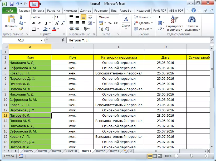
3. As a result of our actions on the "quick access panel" a new icon appeared. Click on it.



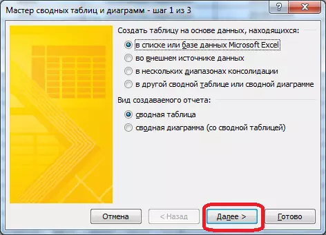
4. After that, the "Summary Wizard" opens. There are four data source options, from where a summary table, from which we specify the appropriate one will be formed. Below should choose that we are going to create: a summary table or chart. We choose and go "Next".



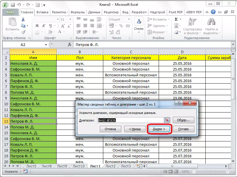
5. A window appears with a data table with data, which can be changed if desired. We do not need to do this, so we simply go to "Next".



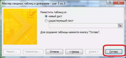
6. Then the "Master of Summary Tables" offers to choose a place where a new object will be located: on the same sheet or on the new one. We make a choice and confirm it with the "Finish" button.



7. A new sheet opens exactly with the same form that was with the usual way to create a pivot table.
8. All further actions are performed on the same algorithm that was described above (see option 1).

Setting up a consolidated table

As we remember from the conditions of the task, the table should remain only for the third quarter. In the meantime, information is displayed for the entire period. Let us show an example of how to make it setting.

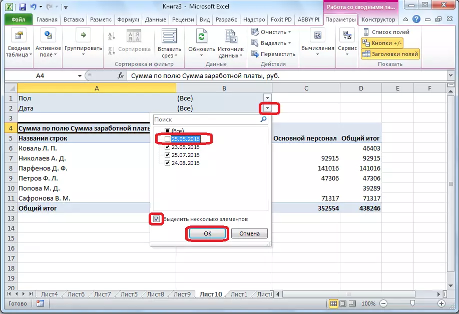
1. To bring the table to the desired view, click on the button near the "Date" filter. In it, we set a tick opposite the inscription "Select several elements". Next, remove the checkboxes from all dates that do not fit into the period of the Third Quarter. In our case, this is just one date. Confirm the action.



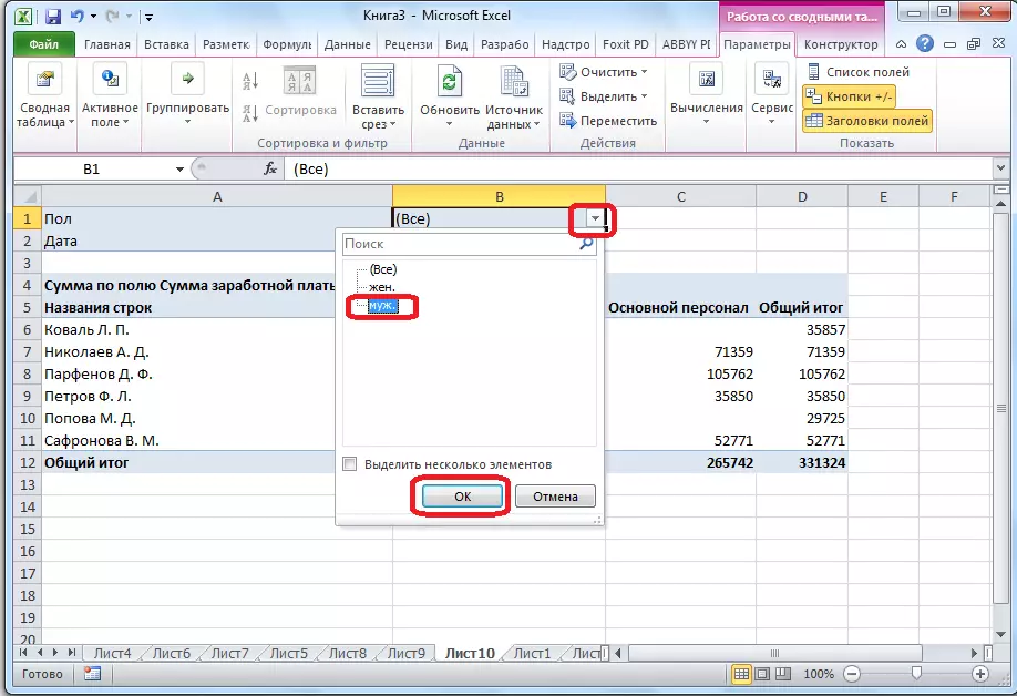
2. In the same way, we can use the filter by the floor and choose for a report, for example, only one men.



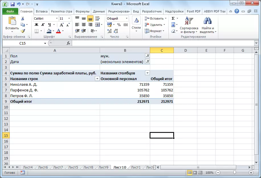
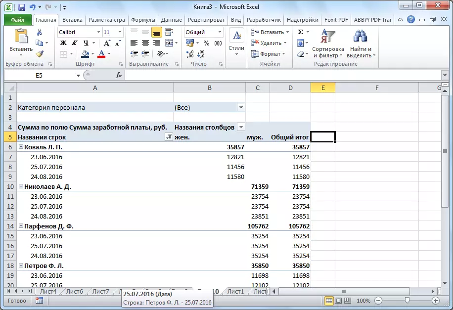
3. The consolidated table acquired this species.



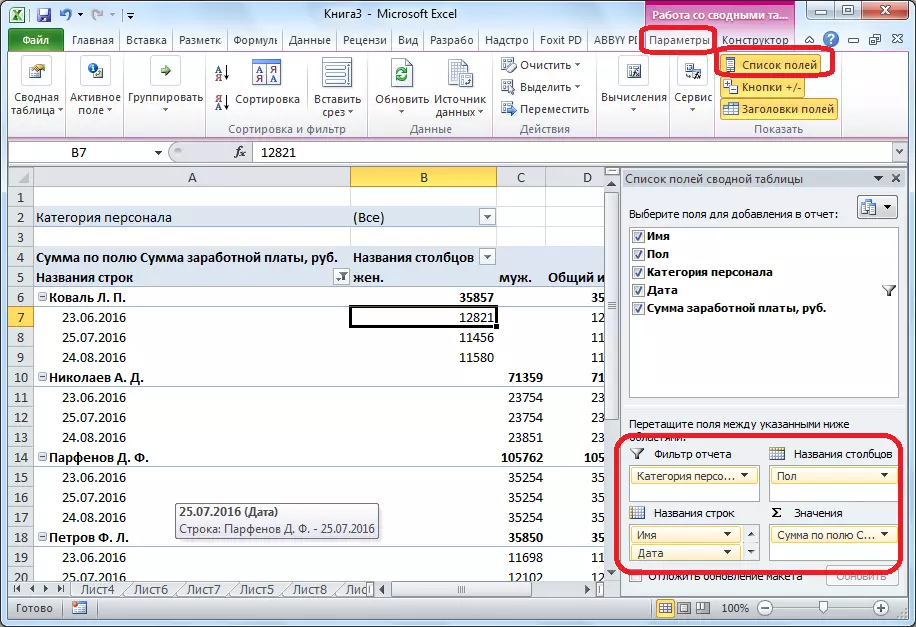
4. To demonstrate that you can manage the information in the table as you like, open the field list form. Go to the "Parameters" tab, and click on the "List of Fields". We move the field "Date" from the Filter of the Report "in the" Line name ", and between the" Personnel category "and" Paul "fields produce the exchange of areas. All operations are performed using simple reliating elements.



5. Now the table looks completely different. The columns are divided by fields, a breakdown of months appeared in the rows, and the filtering can now be carried out by personnel category.



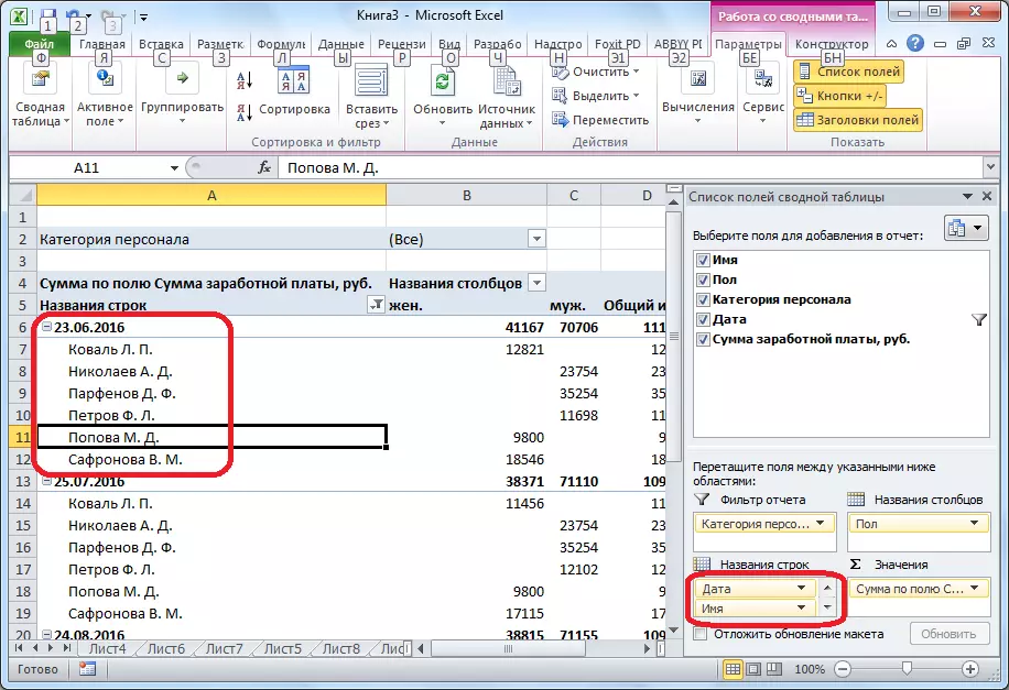
6. If in the list of fields, the name of the strings move and put the date above the date than the name, then it is the payday dates that will be divided into employee names.



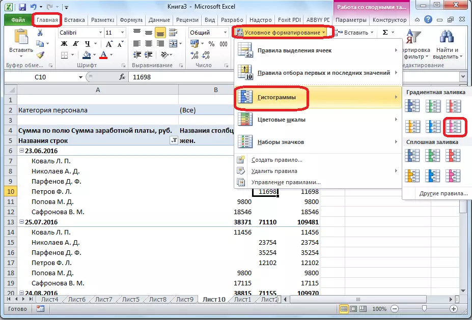
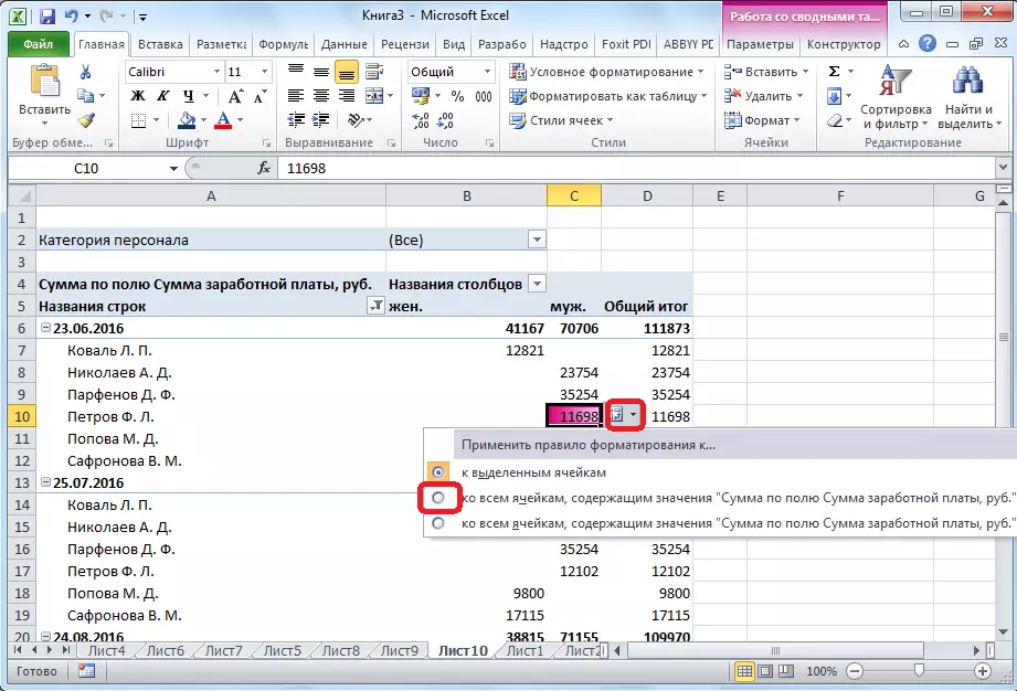
7. You can also display the numeric values ​​of the table as a histogram. To do this, select a cell with a numeric value, we go to the "Home" tab, click "Conditional Formatting", select the item "Histograms" and specify the view like.



8. The histogram appears only in the same cell. To apply a histogram rule for all table cells, click on the button, which appeared next to the histogram, and in the window that opens, we translate the switch to the "To all cells" position.



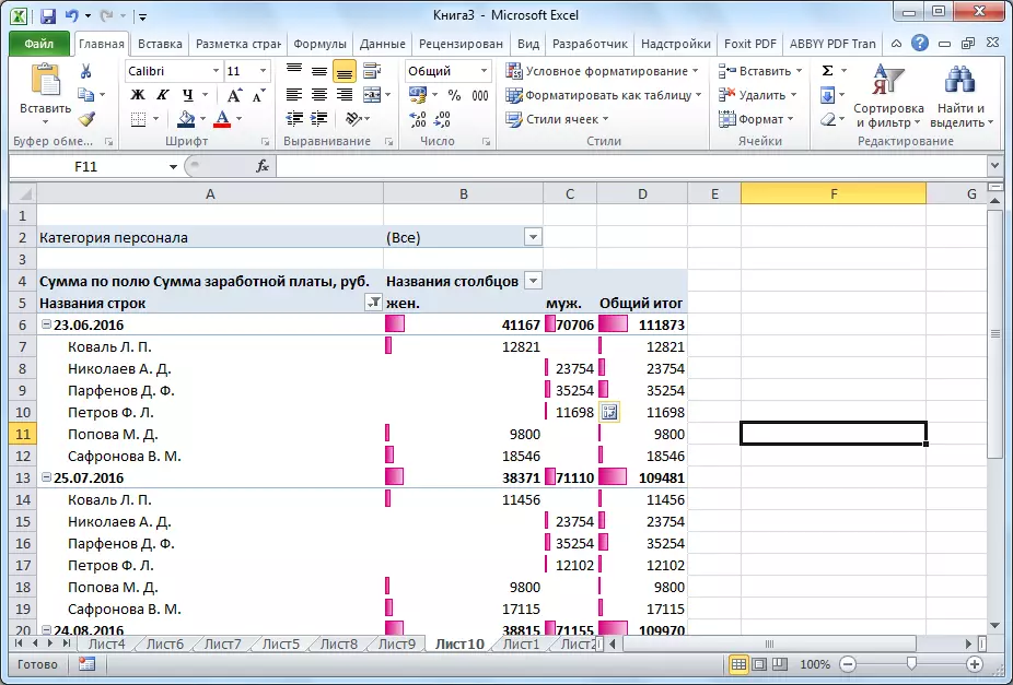
9. As a result, our pivot table began to look more presentable.

The second method of creation provides more additional features, but in most cases the functionality of the first variant is quite enough to perform the tasks. Summary tables can generate data to reports on almost any criteria that the user specifies in the settings.