Function intermediate results in Excel

When working with tables, there are often cases when, in addition to common results, it is necessary to pour and intermediate. For example, in the sales table for a month in which each individual line indicates the amount of revenue from the sale of a particular type of goods per day, you can bother daily intermediate results from the sale of all products, and at the end of the table, specify the value of the total monthly revenue to the enterprise. Let's find out how to make intermediate results in the Microsoft Excel program.

Using the "Intermediate Results" function in Excel

Unfortunately, not all tables and data sets are suitable for applying intermediate results to them. The main conditions are as follows:

• The table must have the format of the conventional area of ​​the cells;
• The table hat must consist of one row and placed on the first line of the sheet;
• The table should not be lines with empty data.

Creating intermediate results in Excel

Go to the process itself. For using this, the tool meets a separate section made to the top panel of the program.

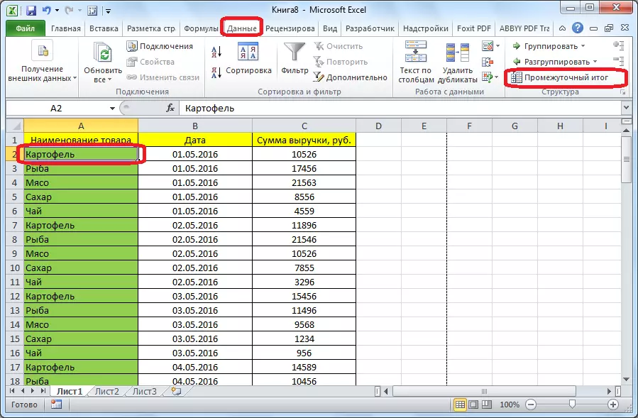
1. Select any cell in the table and go to the Data tab. Click on the "Intermediate Outcome" button, which is located on the tape in the "Structure" tool block.



2. A window will open in which you need to configure the removal of intermediate results. In our example, we need to view the sum of the total revenue for all goods for every day. Date value is located in the column of the same name. Therefore, in the field "With each change in", select the "date" column.
3. In the "Operation" field, we select the value "amount", as we need to fake exactly the day per day. In addition to the amount, many other operations are available, among which you can allocate: the amount, maximum, minimum, work.
4. Since the revenue values ​​are displayed in the "revenue amount, rubles" column, then in the "Add OTG" field, select it from the list of columns of the table.
5. In addition, you need to install a tick if it is not, near the parameter "Replace the current outcome". This will allow when recalculating the table if you do a procedure for calculating the interim outcomes with it not for the first time, do not duplicate the recording of the same results repeatedly.
6. If you put a tick in the "end of the page between the groups" item, when printing each block of the table with intermediate results will be printed on a separate page.
7. When adding a tick opposite the value "Results under the data", the intermediate results will be installed under the string block, the sum of which is wounded in them. If you remove a tick, then they will be shown above the rows. For most, it is more convenient for lines, but the selection itself is purely individual.
8. Upon completion, click on OK.



9. As a result, the intermediate results appeared in our table. In addition, all groups of strings combined by one intermediate result can be collapsed by simply by clicking on the "-" sign on the left of the table opposite the specific group.



10. So you can minimize all the lines in the table, leaving only intermediate and general results visible.



11. It should also be noted that when changing data in the line of the table, the intermediate results will be recalculated automatically.

Formula "Intermediate. Data"

In addition to the foregoing, it is possible to output intermediate outcomes not through the button on the tape, but by calling a special function through "insert a function".

1. After after clicking on the cell, where the intermediate results will be displayed, click the specified button, which is located on the left of the formula string.



2. "Master of Functions" will open, where among the list of functions, we are looking for the item "Intermediate. Duty". We highlight it and click "OK".



3. In a new window, you will need to enter the function arguments. In the Row "function number", enter the number of one of the eleven data processing options, namely:
   • 1 - average arithmetic value;
   • 2 - the number of cells;
   • 3 - the number of filled cells;
   • 4 - the maximum value in the selected data array;
   • 5 - minimum value;
   • 6 - product of data in cells;
   • 7 - standard sample deviation;
   • 8 - standard deviation by the general population;
   • 9 - sum;
   • 10 - sample dispersion;
   • 11 - dispersion by the general population.



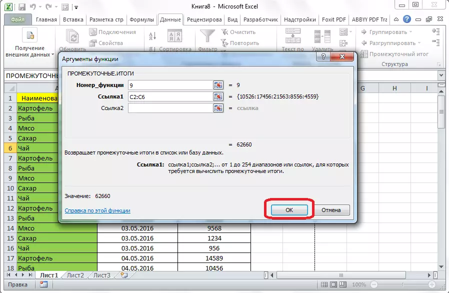
4. In the Count "Link 1", specify the link to that array of the cells for which you want to set intermediate values. It is allowed to introduce up to four scattered arrays. When adding the coordinates of the cell range, a window immediately appears to add the following range. Since it is not convenient to enter the range of manually in all cases, you can simply click on the button located on the right of the input form.



5. The function of the arguments of the function will come and you can simply highlight the desired data array with the cursor. After it is automatically entered into the form, click on the button placed on the right.



6. The function arguments window appears again. If you need to add another or more data arrays, take advantage of the same algorithm that was described above. In the opposite case, simply click OK.



7. Intermediate results of the dedicated range of data will be formed in the cell in which the formula is located.



8. The syntax of the functions itself is as follows: intermediates. These (Function number; address_amissions_dasses). In our situation, the formula will look like this: "Intermediate. Duty (9; C2: C6)". This feature, using this syntax, can be entered into the cells and manually, without calling the "Master of Functions". It is just important not to forget before the formula in the cell to sign "=".

So, there are two main ways to form intermediate totals: through the button on the tape and through a special formula. In addition, the user must determine which value will be displayed as a result: the amount, minimum, average, maximum value, etc.