

Method 1: Editing automatically added block
The first way is the easiest, since it is based on editing the automatically added diagram name. It appears immediately after creating certain graphs or other types of structures, and it will be necessary to make several edits to change.
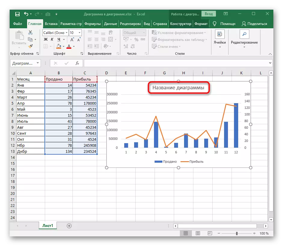
- After creating the diagram, click on the "Diagram Title" row.
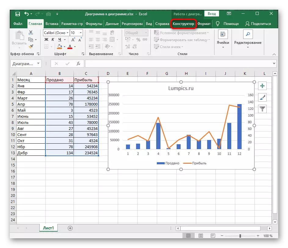
- First, highlight the design itself so that tabs that are responsible for managing it appear on the top of the top.
- Move to the Designer tab.
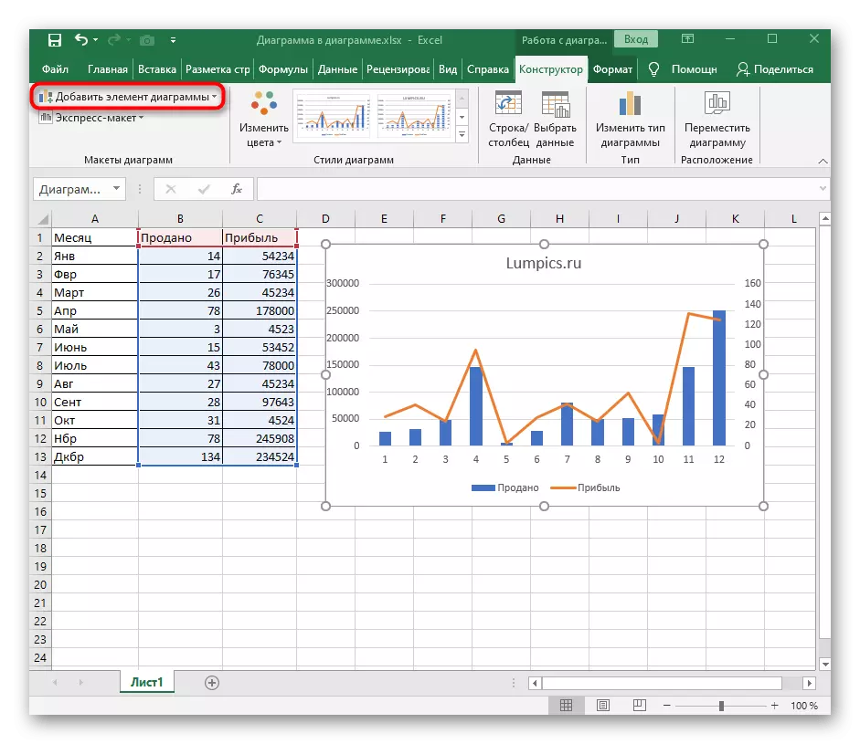
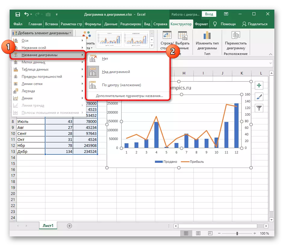
- On the left is the "diagram layouts" block, where you need to deploy the drop-down menu "Add Chart Element".
- Move the cursor to the "Diagram Title" point and select one of the options for its overlay.
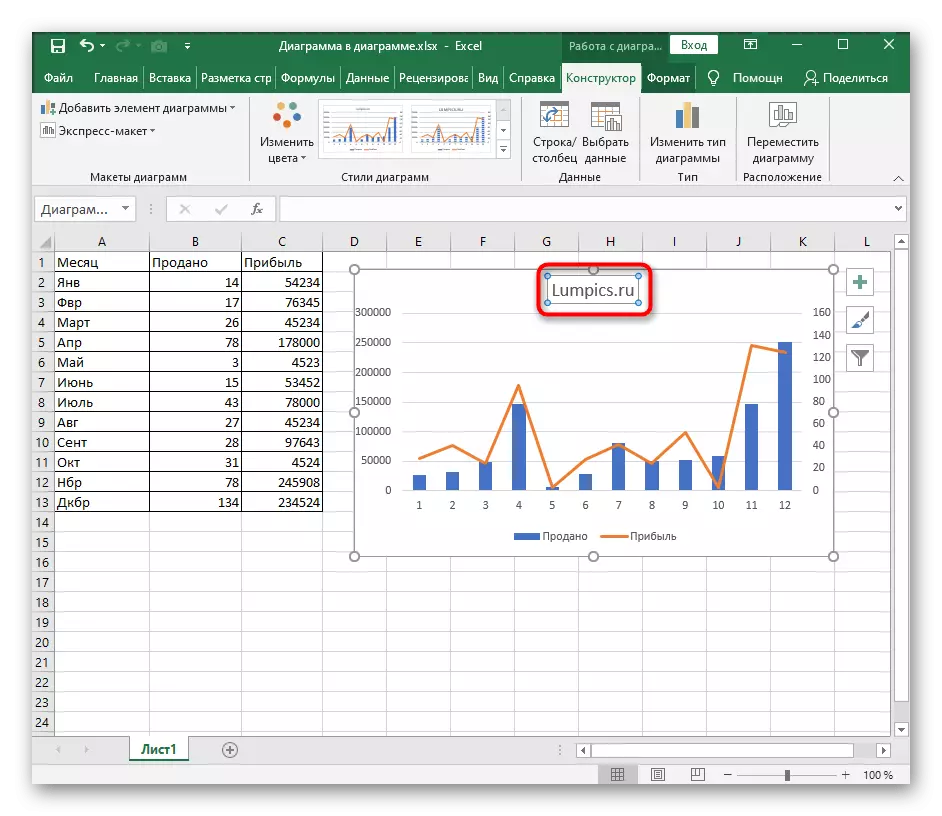
- Now you see the standard display name and you can edit it by changing not only the inscription, but also the format of its display.
- If the diagram name is not at all, use the previous option to create it.
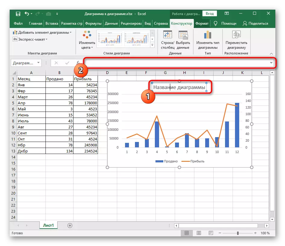
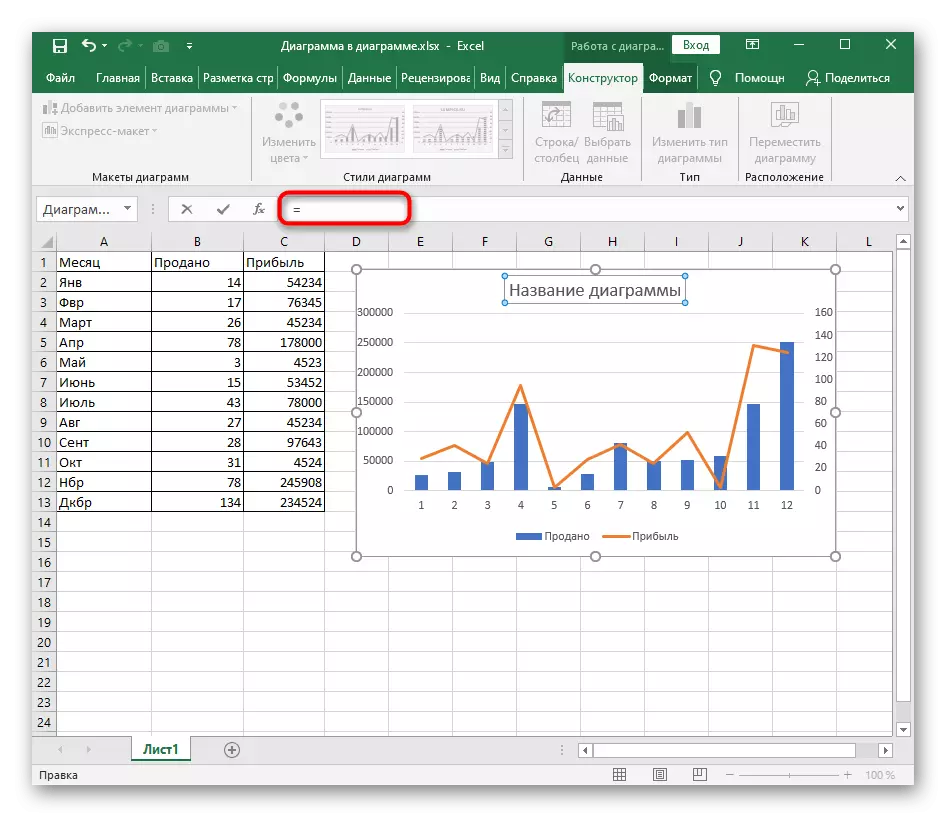
- After that, highlight it for editing, but do not fit any meaning.
- In the line for entering the formula, write a sign =, which will mean the beginning of the automated name.
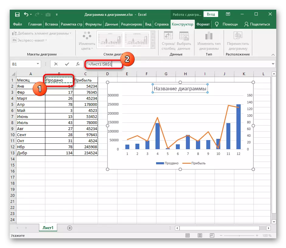
- It remains only to click on the cell, the name of which you want to assign the diagram itself. In the formula input line, the change will immediately appear - press the ENTER key to use it.
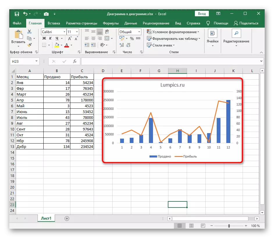
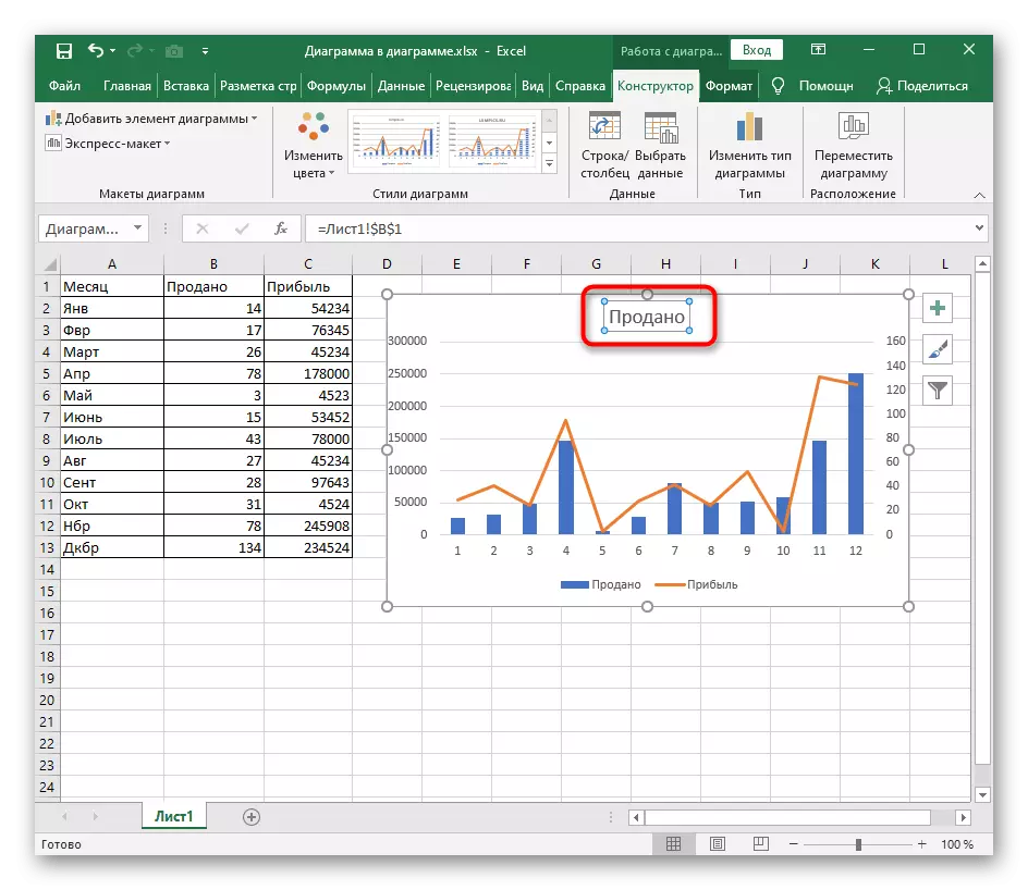
- Check how the diagram name is dynamically changing, editing this cell.
If after creating the diagram, its name was not added automatically or you were accidentally deleted, use the following methods where alternative options are disclosed in detail.
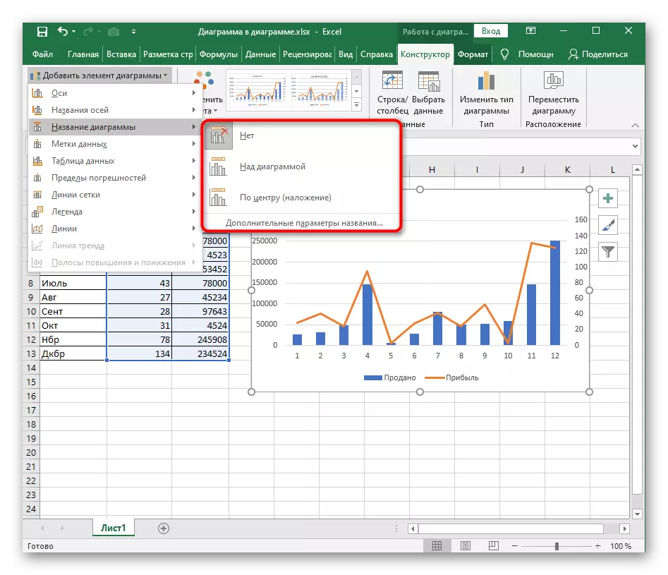
Method 2: Tool "Add Chart Element"
Many users when working with Excel faced the "Designer" tool, designed to edit diagrams and other insertion elements. It can be used for adding a name for less than a minute.
The same method is relevant and for the name of the axes, only in the same drop-down menu should select another item, further editing is carried out in the same way.
Method 3: automated name
The option is particularly useful for users working with tables where the name of the diagram is tied to the name of a particular column or string that sometimes changes. In this case, using the built-in Excel functionality, you can create an automated diagram name assigned to the cell and changing according to its editing.
It is important to inscribe a sign = in a string to edit formulas, and not block name of the chart, because the syntax of the program simply does not work and bind automation will not work.