Examples of the "Smerei" function in Excel

Syntax and function creation

The function is more popular, because in almost every table, it is necessary to calculate the sum of the numbers in the cells, ignoring the values ​​that do not fall under the main condition. Thanks to this formula, the counting does not become complicated and long. The standard design function looks like = silent (range; Criterion; Range_Suming), and the "summation range" is indicated only under the condition where there are actual cells, the addition of which is performed under any circumstances. If the data in the "summation range" is missing, all cells included in the "range" will be checked.

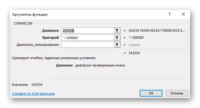
We will analyze the two remaining arguments - the "range" and "criterion". The first fits of the cells (A1: A100) fits (A1: A100), which will be checked and compared with the condition. In the "Criterion", the user brings the condition, when performing the cell becomes one of the terms. This may be the condition of the inequality of numbers (50) or compliance with the specified text ("text"). To simplify the understanding of the installation of arguments, open the graphics window "Argument" and set all the conditions in turn in separate fields.

There are not so many different examples, the features of the filling of which it is worth considering when the function is silent, and then will figure out the basic and most popular.

The function is silent under the condition of inequality

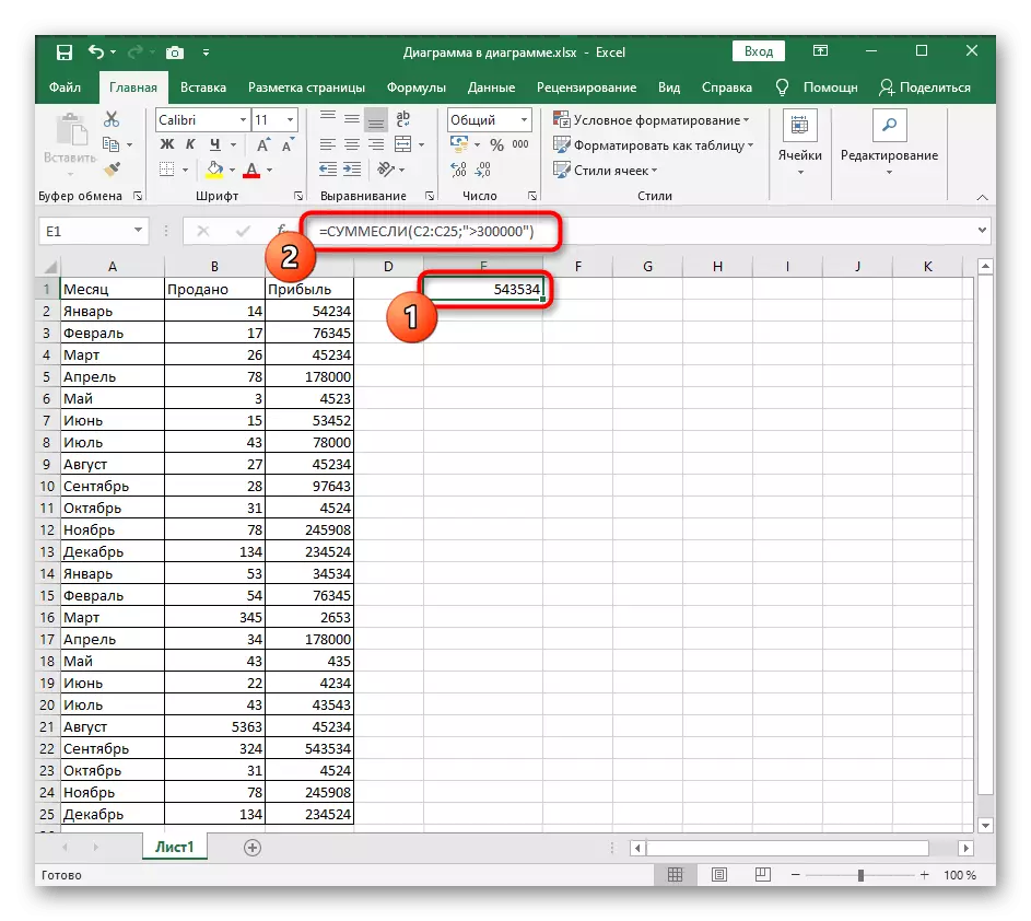
The first example is the use of the function of the function, provided that the number for the hit must be greater, less or not equal to the specified number. With such a syntax, the function checks all cells of the specified range and considers only suitable. Manual writing it through the input field consists of several parts:

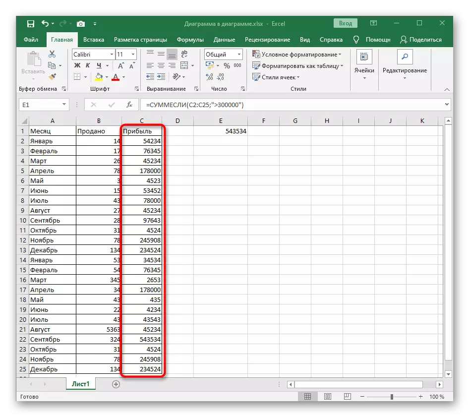
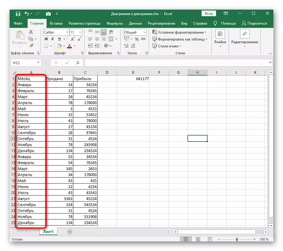
1. Determine the range of cells falling for the formula, we will have a profit for the month.



2. Start an entry from its instructions in the input field by writing themselves.



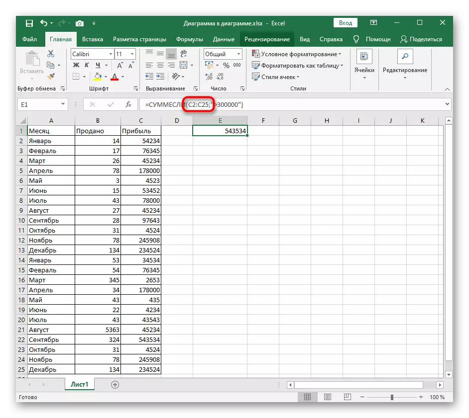
3. Create an opening and closing bracket where you enter the range of selected cells, for example C2: C25. After that, be sure to sign; which means the end of the argument.



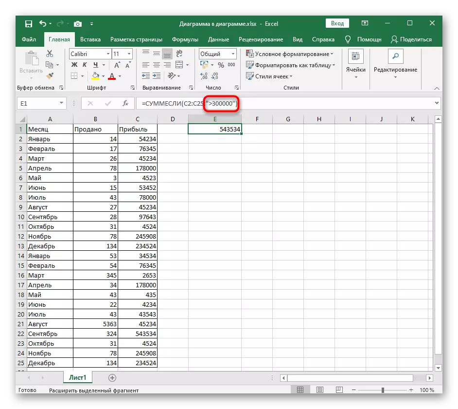
4. Open quotes and specify the condition that in our case will be> 300000.



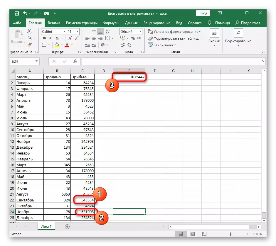
5. As soon as pressing the Enter key, the function is activated. In the screenshot, it is clear that only two cells correspond to the condition> 300000, therefore, the formula summarizes their numbers and displays in a separate block.

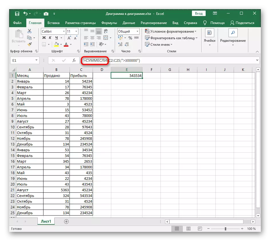
Above, only one of the examples with accidentally taken conditions was disassembled. Nothing will prevent anything to substitute other values, expand or narrow the range - the formula will still normally consider the value if the syntax rules were observed.

The function is silent, subject to matching text

Take the second example when they are silent used to count the amount in cells that are subject to compliance with inscriptions in another range of blocks. This will be useful, for example, when the total price of all goods in one category is calculated, or the company's costs for salaries to employees are calculated on specific positions. An example of registration in this situation is still interesting to the fact that the syntax changes slightly, since the condition falls the second range of cells.

1. This time, in addition to the range of summable cells, determine those where there are inscriptions in the condition.



2. Start recording a function from its designation in the same way as it has already been shown above.



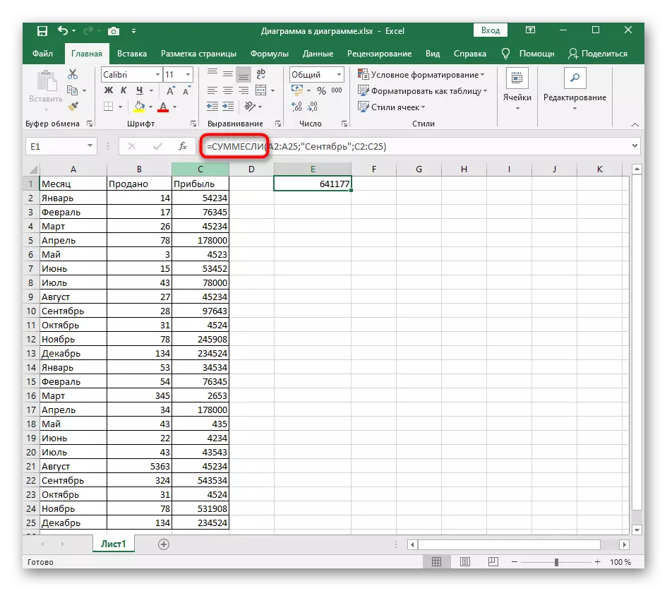
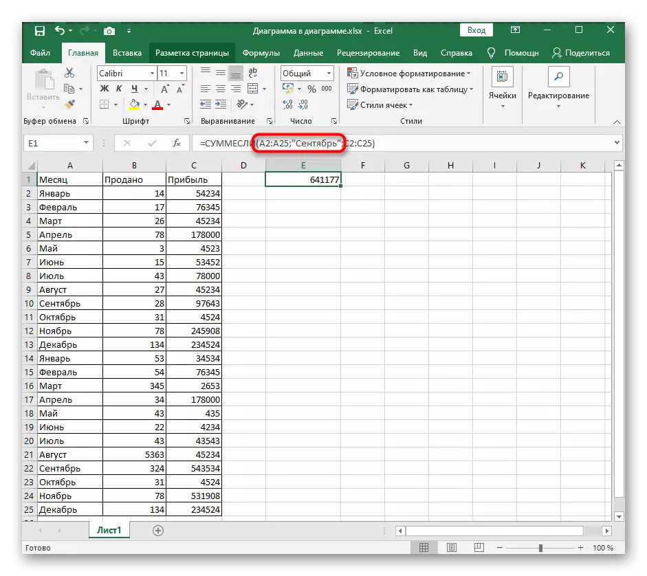
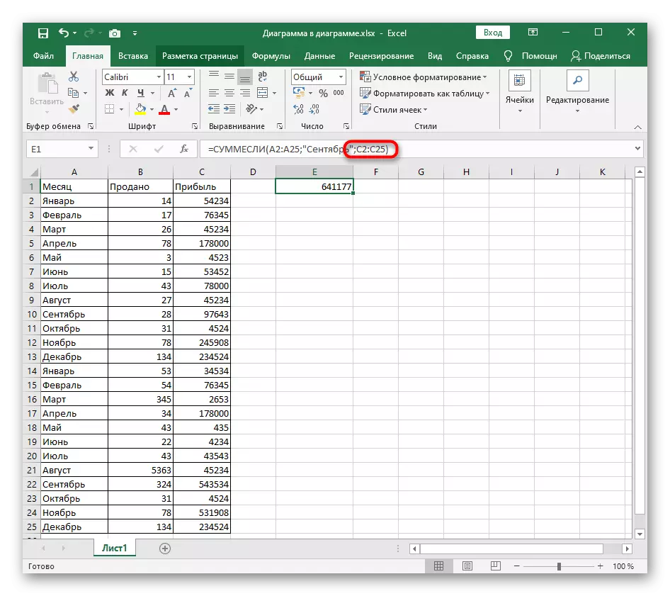
3. First, enter the lapse of the inscriptions, put; And set the condition. Then this expression in the syntactic format will gain approximately this type: A2: A25; "September";



4. As the last argument, it remains to specify the range of cells, the number of which will be summed at the right condition. You are already familiar with the rules for recording such an argument.



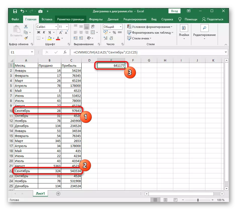
5. Check the action function. We specify the month of September as a condition and look at the table, which summed up two values ​​of table cells that correspond to it. The remaining data when checking is simply ignored.

Replace the word or enter the whole phrase, given the symbol register to create themselves when counting the required values.

Function Smerevilm with several conditions

We completed the analysis of the examples by the third option, when the conditions for adding several at once. With such calculations, the function under consideration is replaced with a modified svmemalimn, which allows you to set more than one argument, which cannot be implemented in the first version. One of the simplest examples with full syntactic correspondence is created as follows:

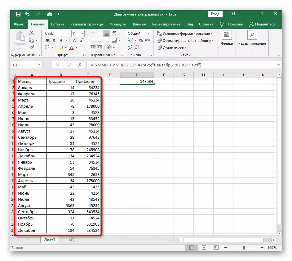
1. Take the table in which there are three different values ​​both on the data there and according to their types. This is a month, the overall profit and the number of goods sold. In a formula with several conditions, it is necessary to make only those profit results, which were obtained in September with sales above 29 units.



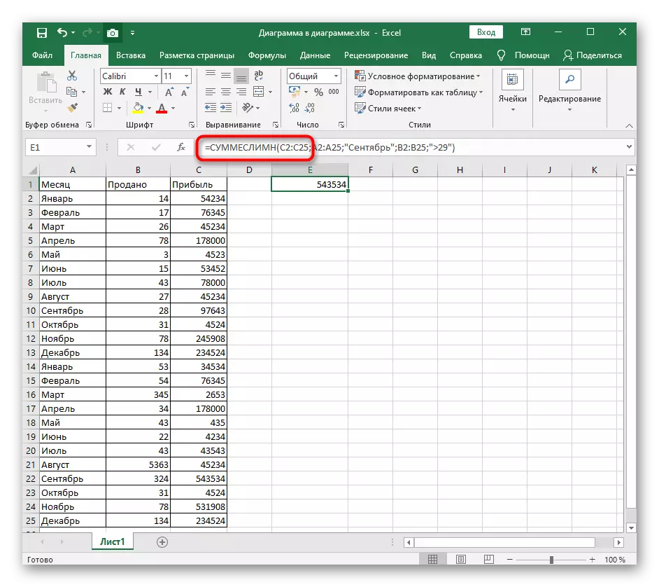
2. Start an entry from the standard ad = Smeremullime, open the brackets and write which range of cells will be summed up. Do not forget to close the announcement of the argument sign;



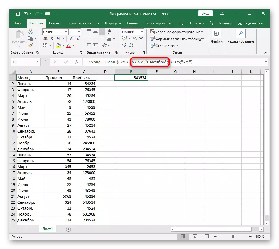
3. Following the second argument - coincidence by name in the cell. The recording of this parameter was already considered above and it can be seen again in the screenshot.



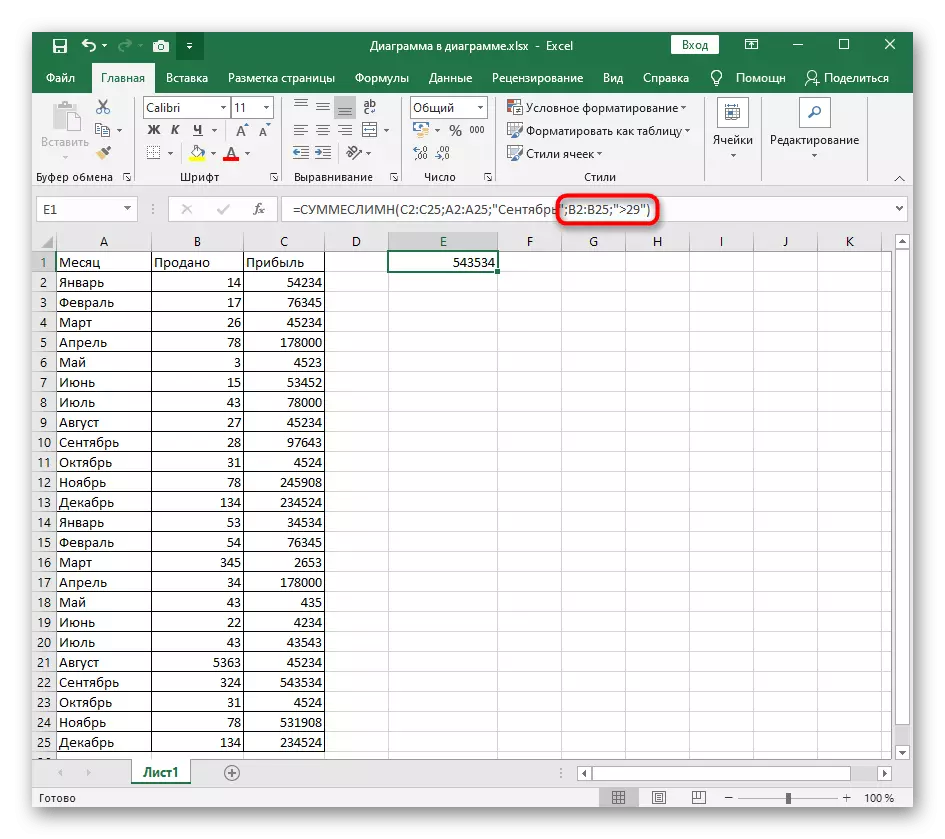
4. The third condition is the correspondence of the predetermined inequality, with which we have familiarized themselves at the beginning of the article. Again in the same format, specify the range of values ​​and the inequality itself in quotes. Do not forget to put the closing bracket, thereby completing the writing function.



5. Fully, the line of this function has the form = svumpremullime (C2: C25; A2: A25; "September"; B2: B25; "> 29"), but you can only adjust it to yourself and get the right result. It may seem that it is difficult to declare each argument and not get confused in the characters, but with a separate approach there should be no problems.

They also sighs and svumpremulls belong to mathematical functions that have a similar syntactic representation, but are used in different situations. To read information on all popular formulas in Excel, refer to the reference material below.

Read more: 10 popular Mathematical functions Microsoft Excel