How to sort by alphabet in Excel

Method 1: Quick Sort Buttons

Excel has buttons responsible for quick sorting of a dedicated data array. Their use will be optimal in those situations when the cells need to be processed only once, having previously allocated the necessary.

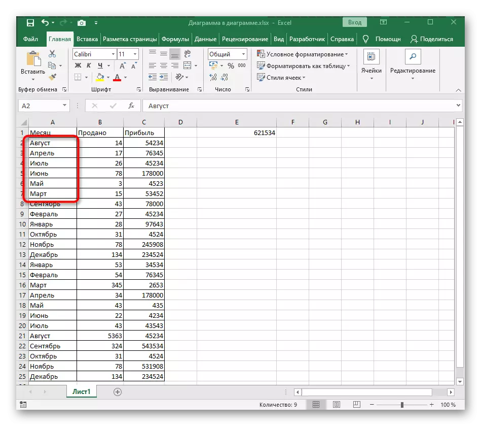
1. Hold the left mouse button and select all the values ​​that will further be subject to sorting.



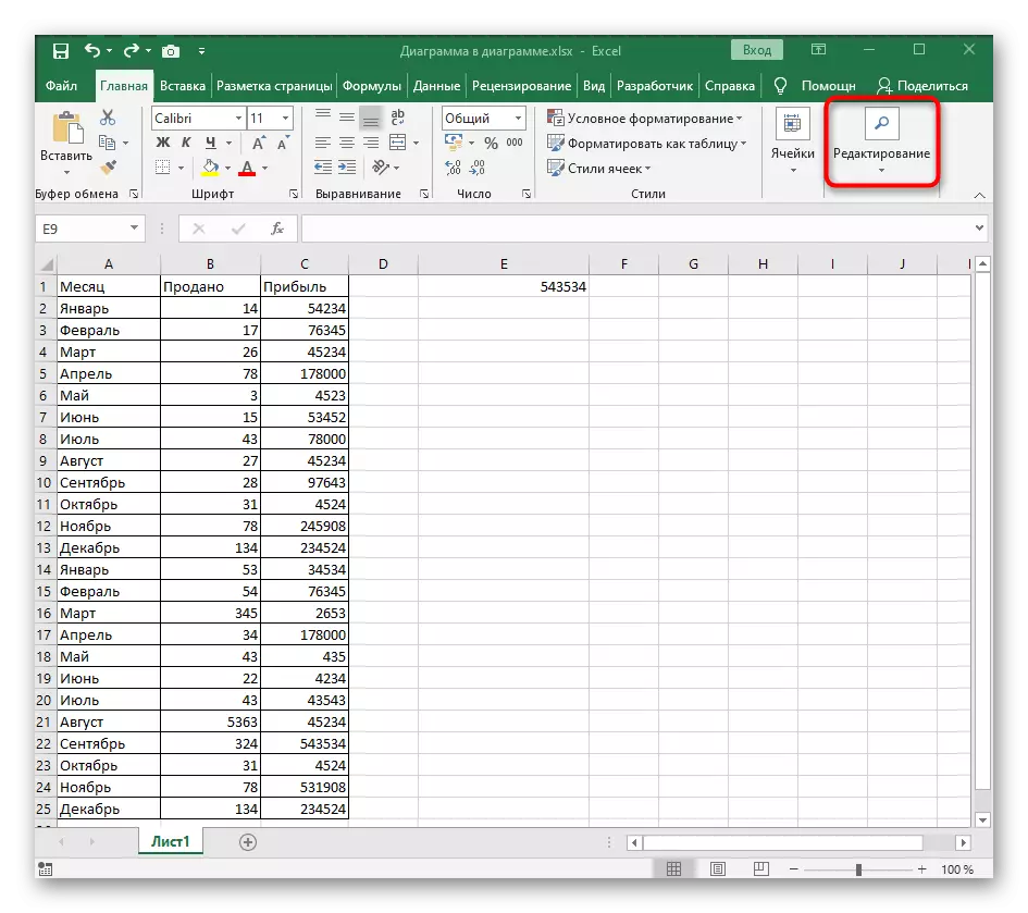
2. On the Home tab, open the "Editing" drop-down menu.



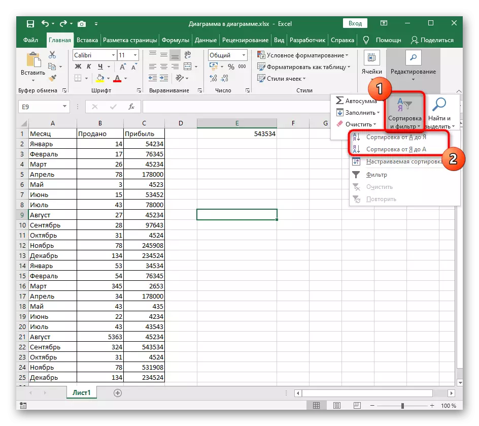
3. In it, use the "Sort and Filtering" block by selecting the order in which you want to place the values.



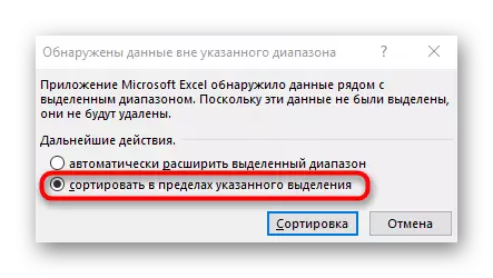
4. If an alert on detecting data out of range appears, you will need to select, expand it or sort only within the specified selection. Consider first the first option.



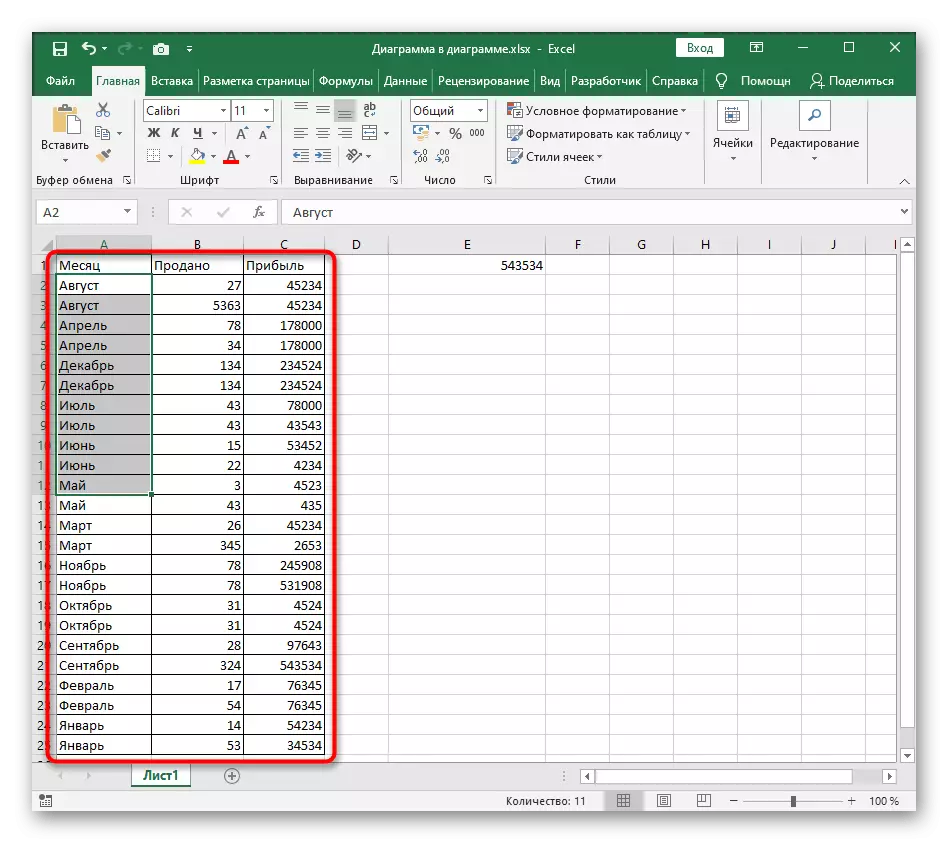
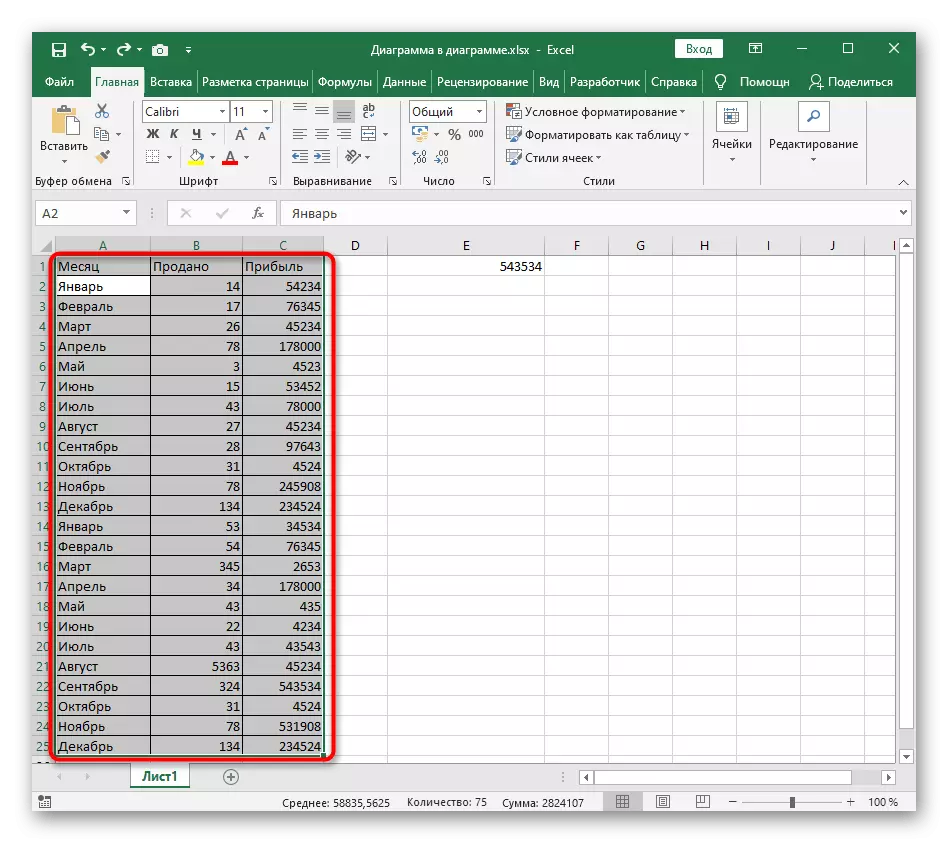
5. When using it, adjacent cells depending on the common table are adjusted under the order of the text layout, that is, if in front of the cell "August" is the value "27", it remains opposite the same word.



6. The second option is to "sort within the specified selection."



7. So only the specified text is moved, and the cells opposite it remain intact. This means that the data displacement will occur if there was some connection before between them.

If you have not yet decided if you want to sort only the specified range or you need to capture the neighboring cells, check each option by pressing it by pressing the Ctrl + Zhe key. It is easier to determine the changes occurring in the table.

Method 2: Customizable Sorting

Customizable sorting allows you to more flexibly build the location of the elements in the table, given several levels and different data ranges. To create it, a special menu is used, which we take into account further.

1. We recommend immediately allocate the entire table if in addition to the sorting alphabet you wish to add a few more levels.



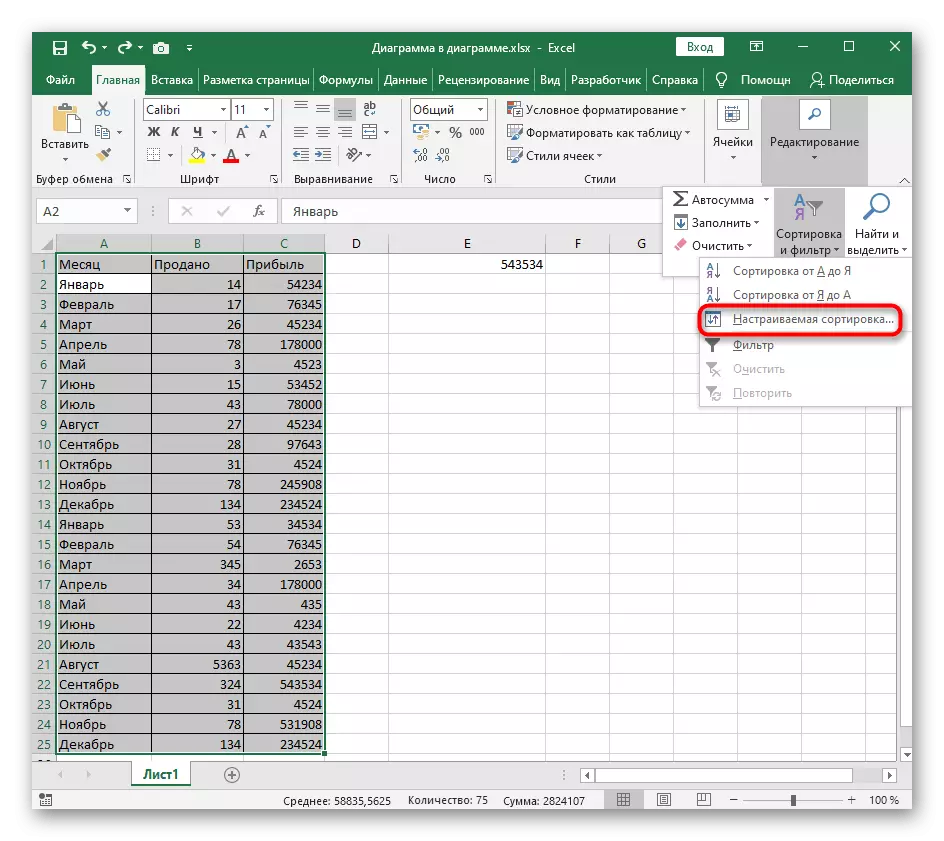
2. Then, in the same section "Editing", choose the item "Customizable Sorting".



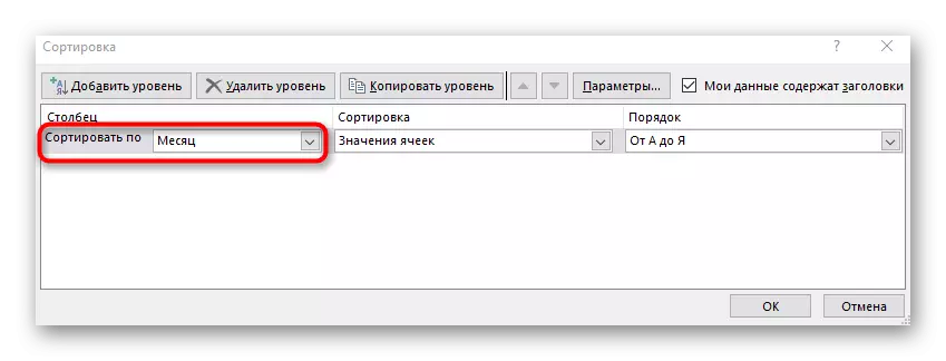
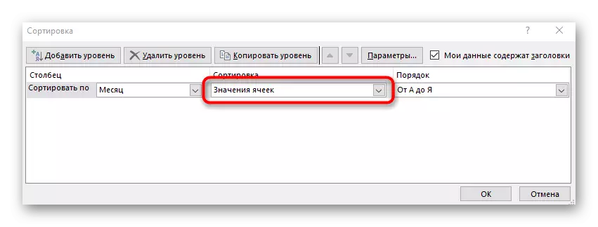
3. In the drop-down menu "Sort by", specify a column that affects the sorting.



4. The type of "cell values" is selected as the sort mode.



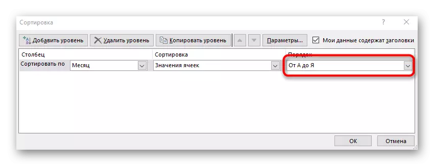
5. It remains only to indicate the order "from A to Z" or "from I up to A".



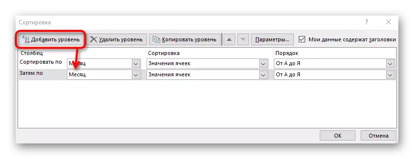
6. If you need to sort and other columns, add them as levels and perform the same setting.



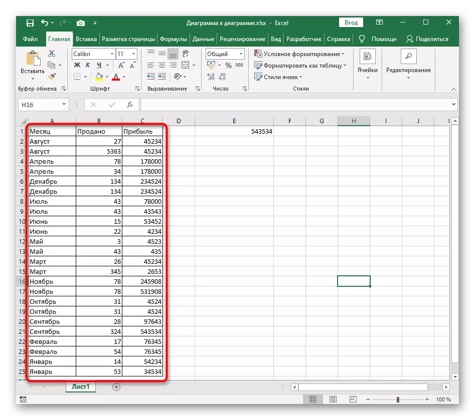
7. Return to the table and make sure all actions are configured correctly.

Method 3: Sort Formula

The disadvantages of previous methods are that they only assort the one-time, and dynamically the table does not change when changes. If you do not suit this option, you will need to manually create a sorting formula that, when adding or removing items, it automatically recalculates them and put in the desired order. The formulas will be somewhat, since so far the developers have not added a special function that would make it without applying the auxiliary calculations. The entire further process consists of several stages to properly understand the principle of sorting according to the alphabet.

Step 1: Creating auxiliary formula

The main task is to create an auxiliary formula that analyzes words in the cells and defines their sequence number in the future sorted by the alphabetic list. This occurs when compared with the embedded Excel algorithms operating on the principle of encoding analysis. In detail to disassemble the work of this formula, we will not only show its creation.

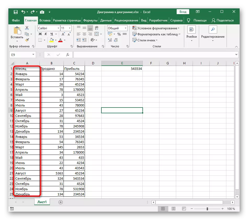
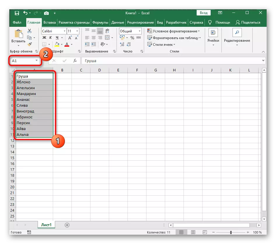
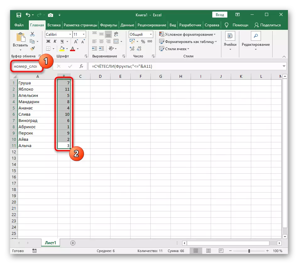
1. To work with future computing, you will need to create a group from cells, for which they need to be allocated and in a specially designated field from above set a new name.



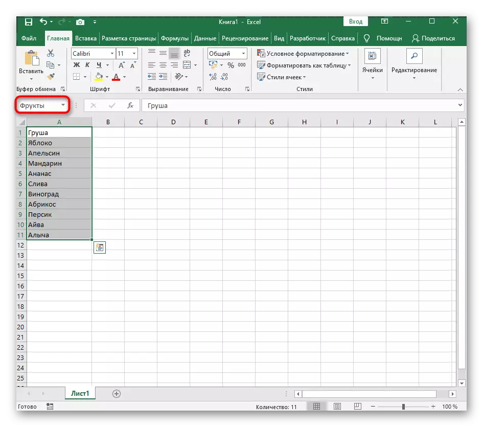
2. Now the range of selected cells has its own name that is responsible for its contents - in our case it is fruits. If you enter a few words in the title, do not put space, but use the lower underscore instead: "(example_text)."



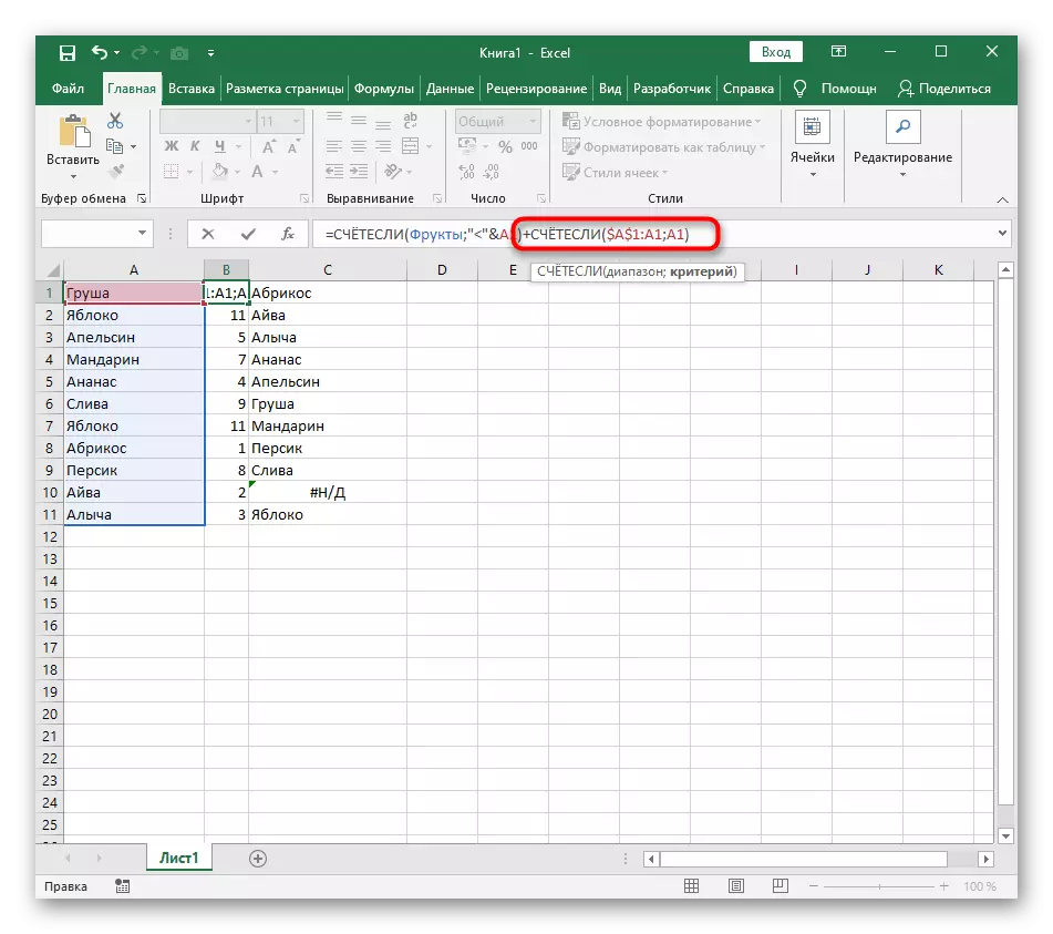
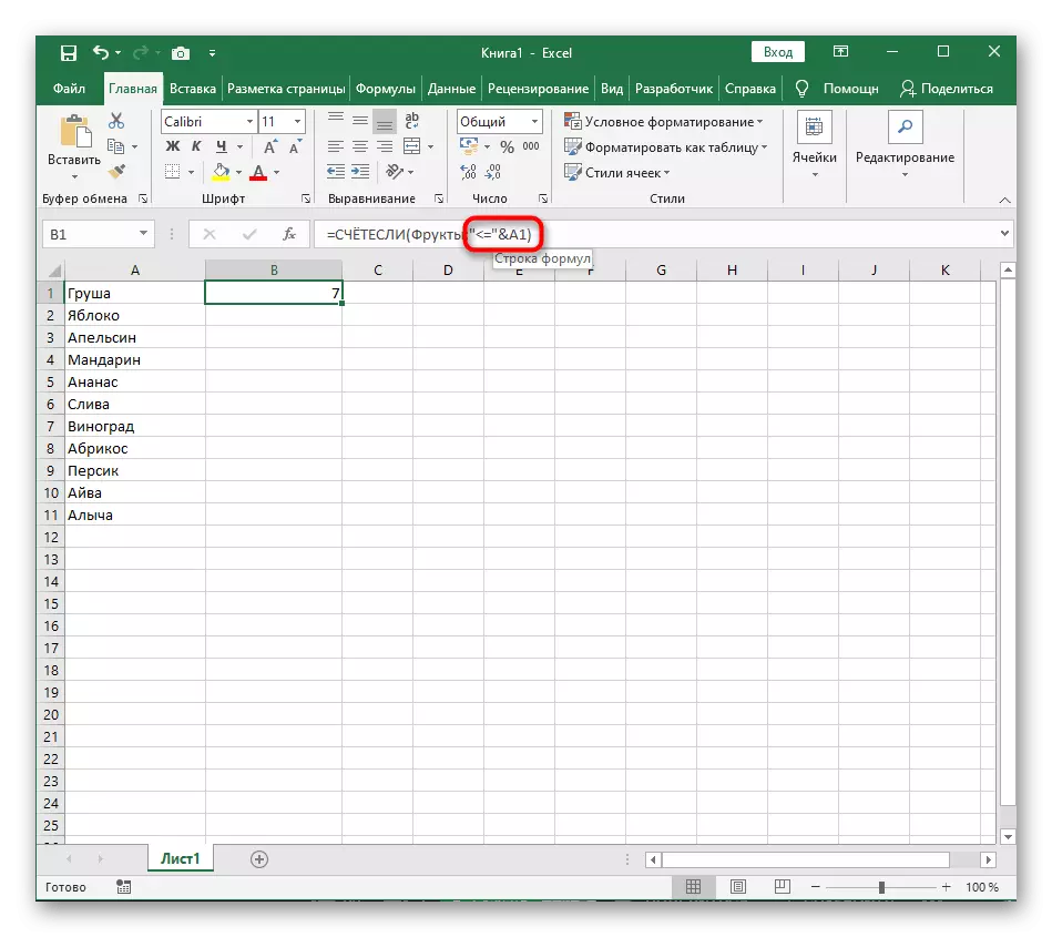
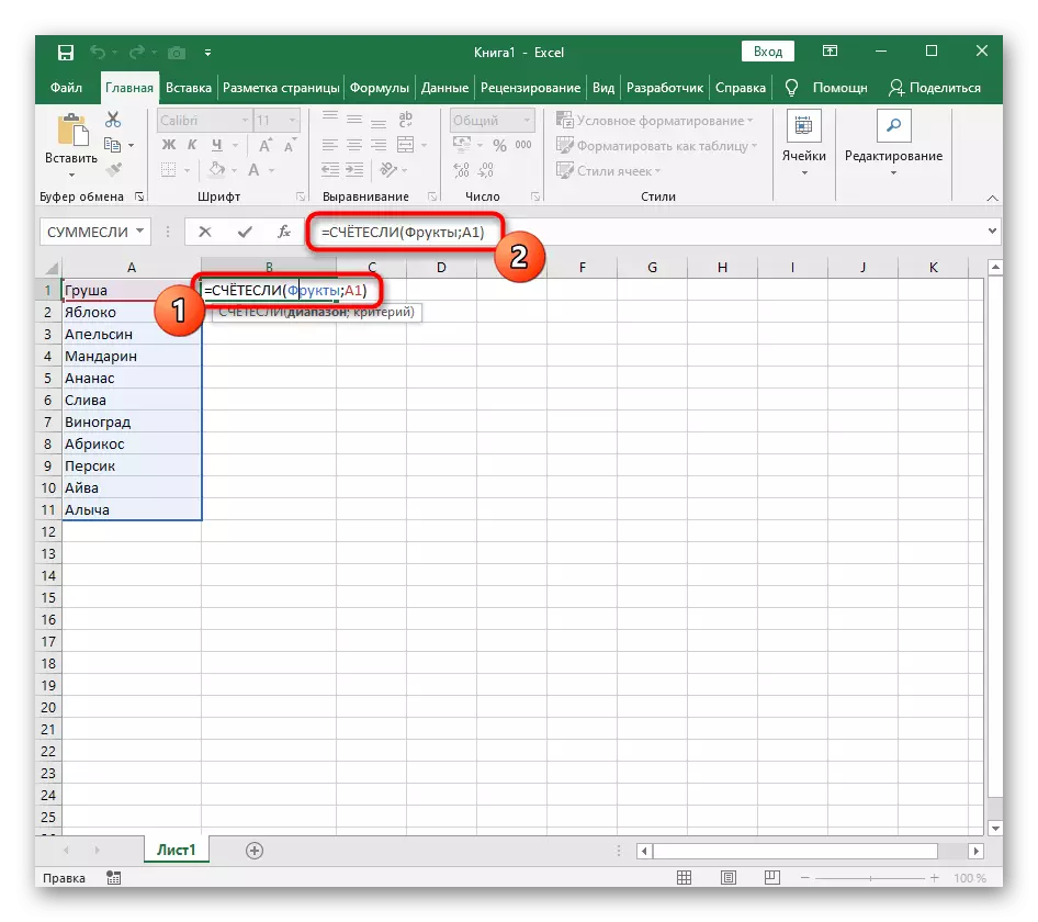
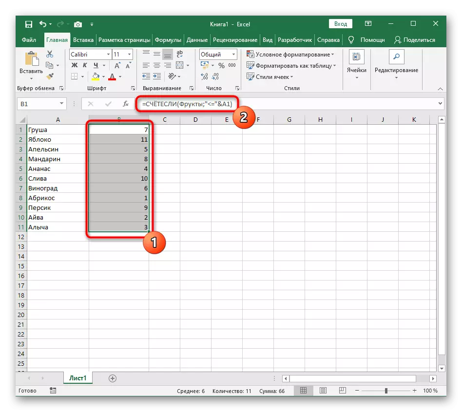
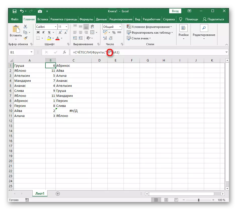
3. In the new cage, we will create a formula of the account, which considers cells satisfying the condition. As a range, specify the newly created group, then the first cell for comparison. As a result, the initial type of formula is: = counted (fruit; A1).



4. Now the result of this formula will be "1", since its record is not entirely true for future settlements, so add an expression "

   

5. Stretch the formula, clinging the edge of the cell, until the end of the future list for sorting.



6. Rename the range with the groups in the group - it will be necessary when drawing up the following formula.

Step 2: Creating a sorting formula

The auxiliary formula is ready and works correctly, so you can proceed to creating a basic function, which will be engaged in sorting thanks to an existing automatic position identifier.

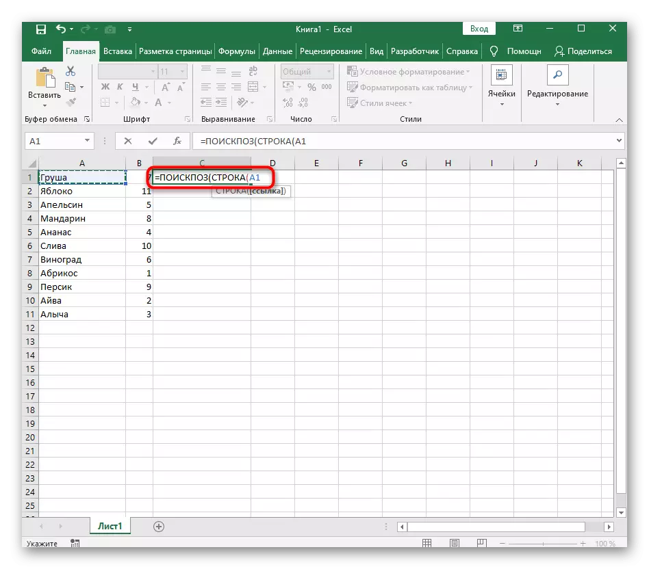
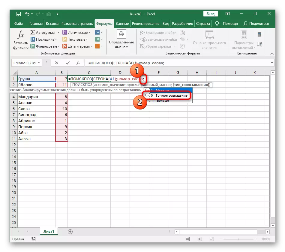
1. In the new cell, start entering = search board (string (A1). This formula is responsible for finding the position position, which is why the argument "A1" should be specified.



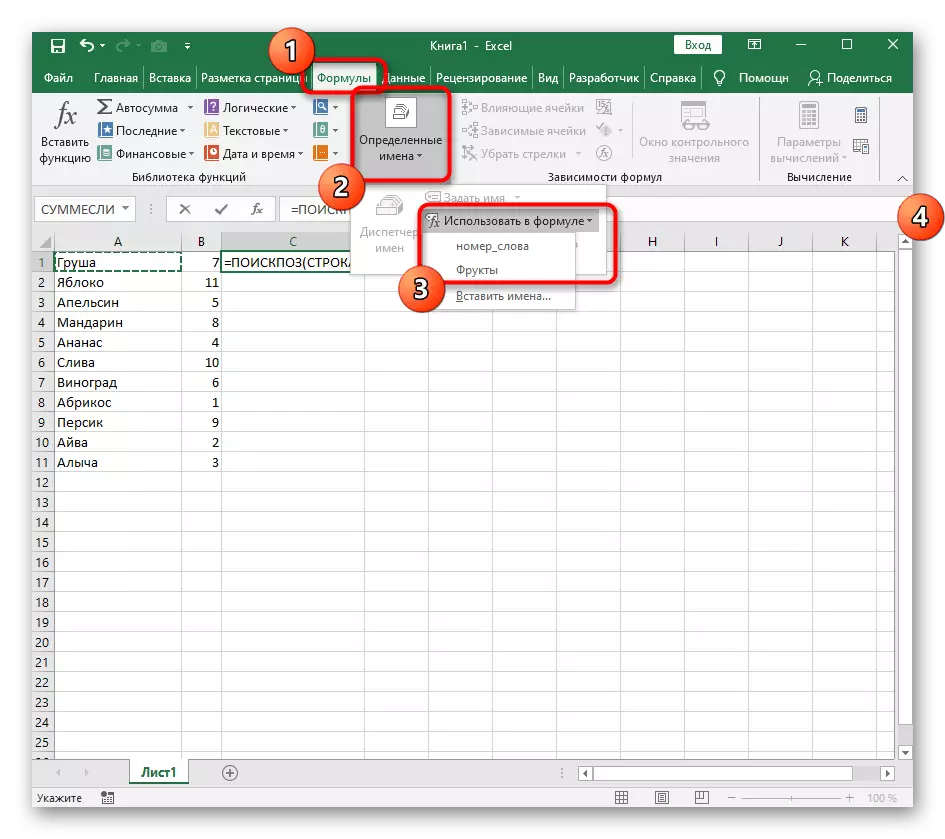
2. Next, to simply add named ranges, go to "Formulas", expand the "Certain Names" menu and select "Use in the formula".



3. Add a range with auxiliary formula and specify a "accurate match" mapping type for it in the drop-down list, which will appear after adding ";".



4. Complete the creation of a formula that wrapped it into the index function that will work with the array of titles.



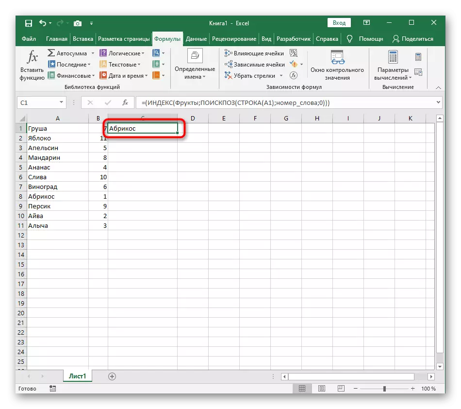
5. Check out the result and then stretch the formula as it has already been shown above.



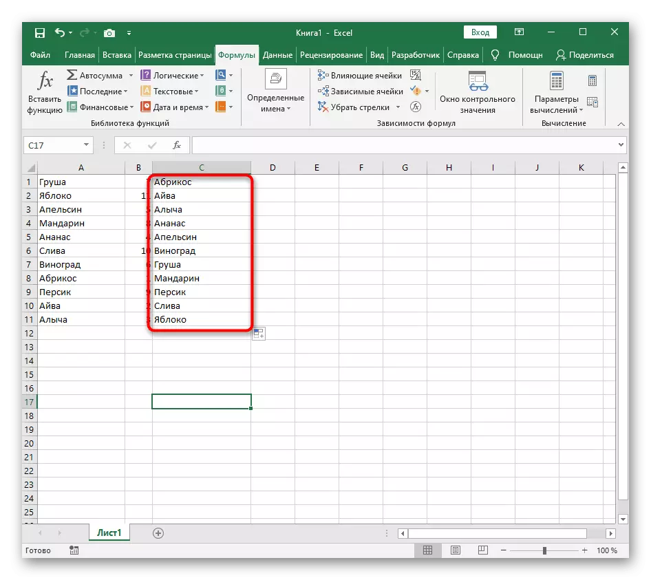
6. Now you will receive a correctly working dynamic list sorted by alphabet.

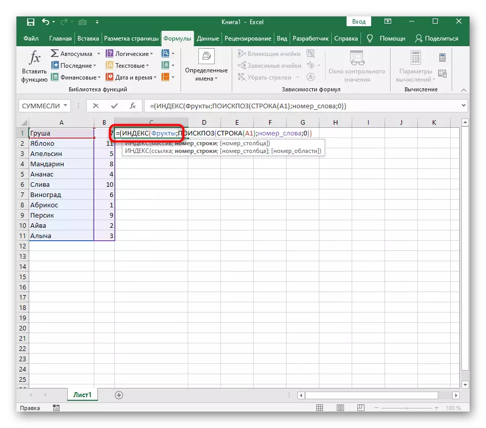
To simplify understanding, separately provide a full formula:

= (Index (fruits; search board (line (A1); number__lov; 0))), you will also remain to edit it under your goals and stretch to the desired range of cells.

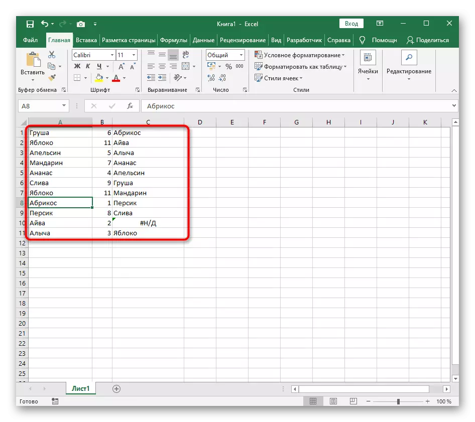
Step 3: Modeling formula for repeated names

The only drawback of the newly created formula is incorrect work in the presence of repeated names that you can see on the screenshot presented below. This is due to the fact that the auxiliary function is not able to correctly process repeating words, so it will have to be improved a little if you want to use the repetitions in the list.

1. Open the auxiliary formula and remove the sign "

   

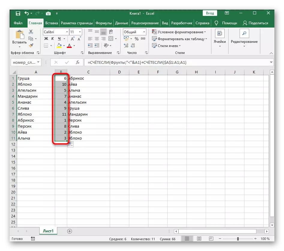
2. Add the second part - + counted ($ A $ 1: A1; A1), allowing you to write the same words in a sequential order normally.



3. Stretch the formula again so that it changed on all cells.



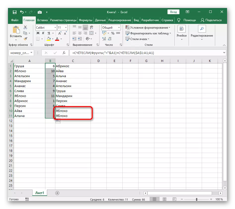
4. Add the duplicate name to the list to check their normal display.