How to draft text in Excel

Method 1: Using an automatic tool

Excel has an automatic tool designed to split text in columns. It does not work automatically, so all actions will have to be done manually, selecting the range of processed data. However, the setting is the most simple and fast in the implementation.

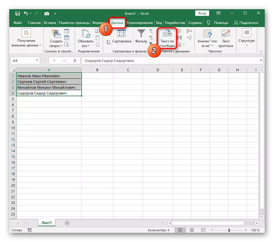
1. With the left mouse button, select all the cells whose text you want to divide on the columns.



2. After that, go to the Tab "Data" and click the "Text to Column" button.



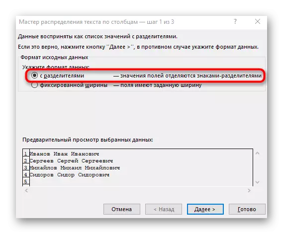
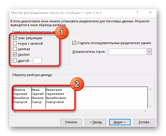
3. The "Column Text Wizard" window appears, in which you want to select the data format "with separators". The separator most often performs space, but if this is another punctuation sign, you will need to specify it in the next step.



4. Tick ​​the sequence symbol check or manually enter it, and then read the preliminary separation result in the window below.



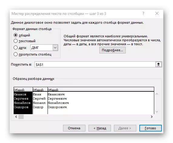
5. In the final step, you can specify a new column format and a place where they must be placed. Once the setup is completed, click "Finish" to apply all changes.



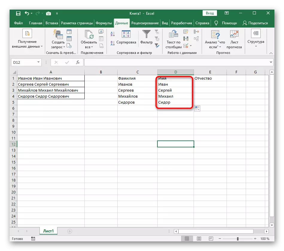
6. Return to the table and make sure that the separation has passed successfully.

From this instruction, we can conclude that the use of such a tool is optimally in those situations where the separation must be performed only once, denoting for each word a new column. However, if new data is constantly introduced into the table, all the time to divide them will this way be not quite convenient, so in such cases we suggest familiarizing yourself with the following way.

Method 2: Creating a text split formula

In Excel, you can independently create a relatively complex formula that will allow you to calculate the positions of words in the cell, find gaps and divide each into separate columns. As an example, we will take a cell consisting of three words separated by spaces. For each of them, it will take their own formula, therefore we divide the method into three stages.

Step 1: Separation of the first word

The formula for the first word is the simplest, since it will have to be repelled only from one gap to determine the correct position. Consider each step of its creation, so that a complete picture formed is why certain calculations are needed.

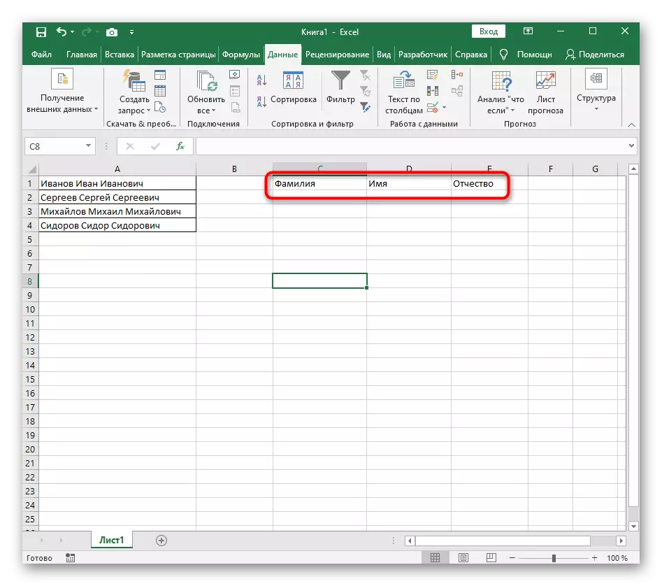
1. For convenience, create three new columns with signatures where we will add separated text. You can do the same or skip this moment.



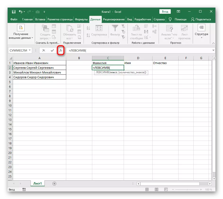
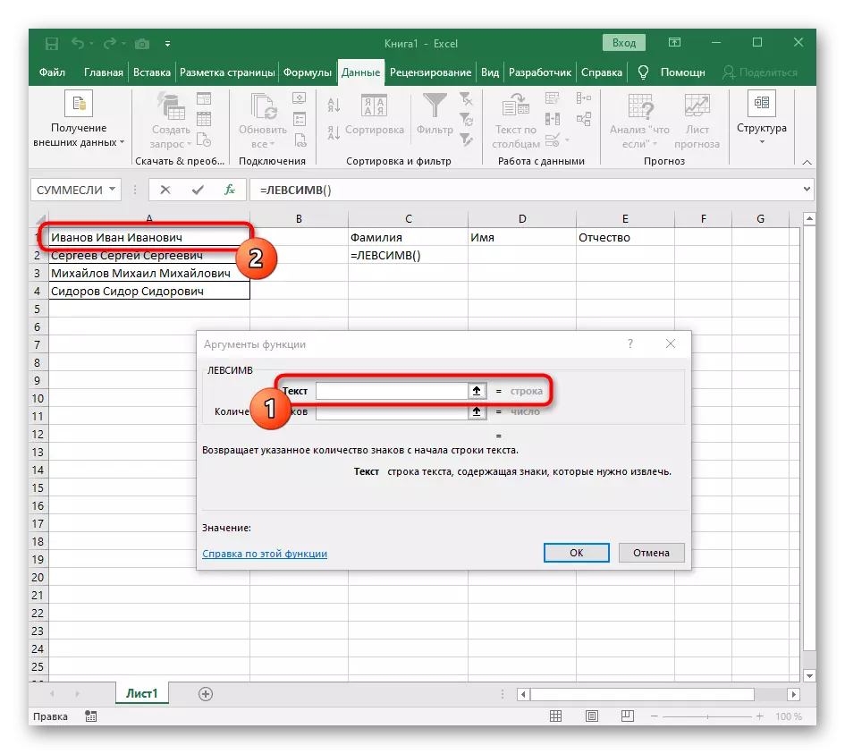
2. Select the cell where you want to position the first word, and write down the formula = Lessimv (.



3. After that, press the "Option Arguments" button, thus moving into the graphic editing window of the formula.



4. As the text of the argument, specify the cell with the inscription by clicking on it with the left mouse button on the table.



5. The number of signs to a space or another separator will have to calculate, but manually we will not do this, but we will use another formula - search ().



6. As soon as you record it in such a format, it will appear in the text of the cell on top and will be highlighted in bold. Click on it to quickly transition to the arguments of this function.



7. In the "Skeleton" field simply put the space or the separator used because it will help you understand where the word ends. In the "Text_-search" specify the same cell being processed.



8. Click on the first function to return to it, and add at the end of the second argument -1. This is necessary in order for the search formula to take into account not the desired space, but the symbol to it. As can be seen in the following screenshot, the result is displayed without any spaces, which means that the formula compilation is made correctly.



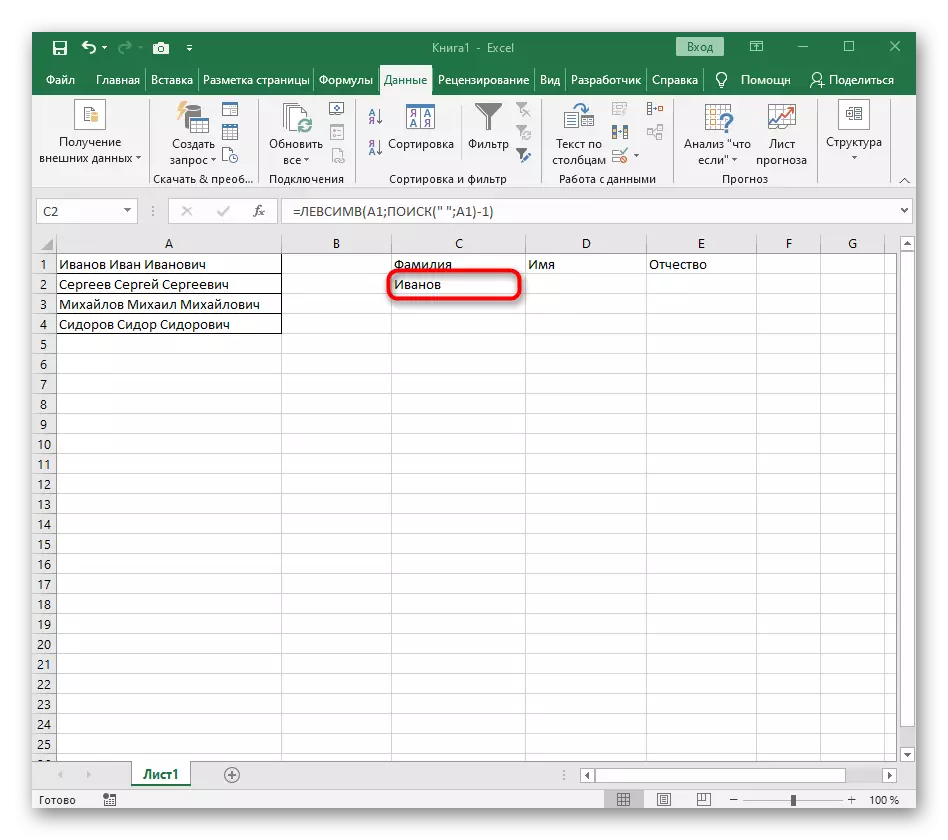
9. Close the function editor and make sure that the word is correctly displayed in the new cell.



10. Hold the cell in the lower right corner and drag down to the required number of rows to stretch it. So the values ​​of other expressions are substituted, which must be divided, and the fulfillment of the formula is automatically.

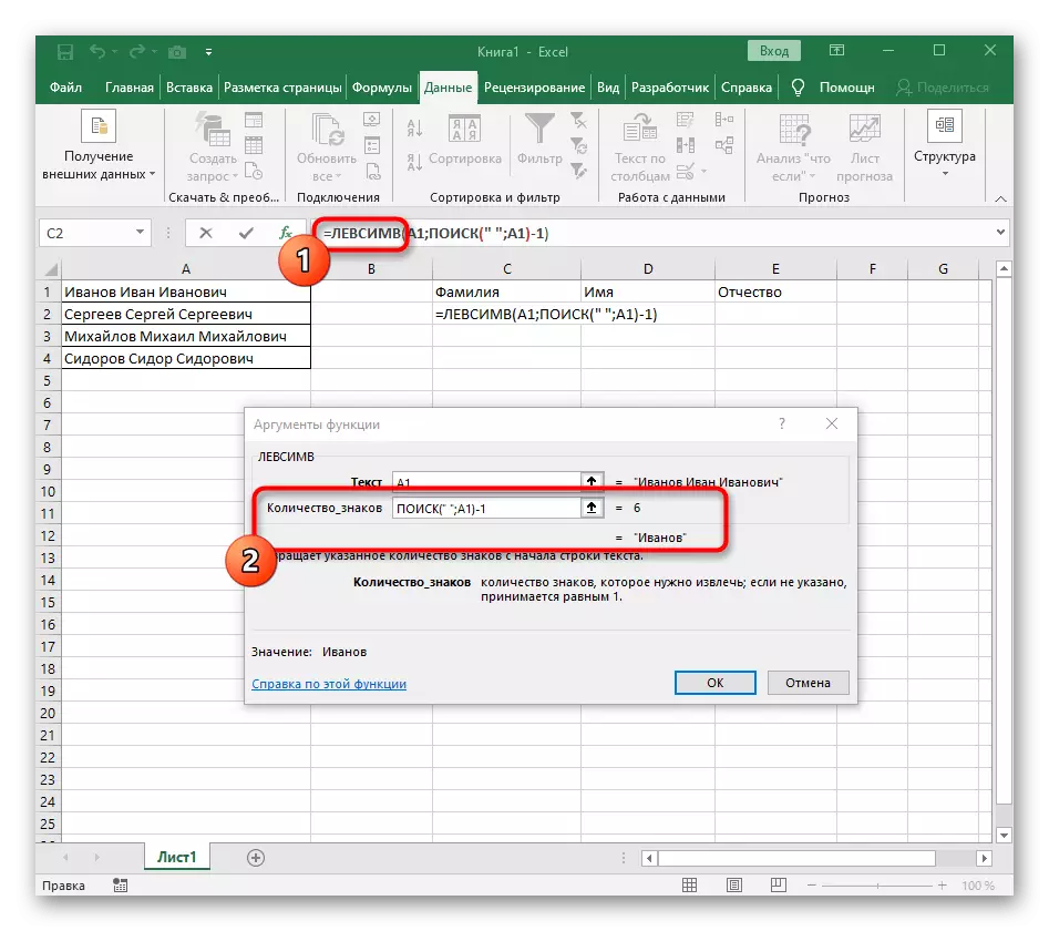
The fully created formula has the form = Levsimv (A1; search (""; A1) -1), you can create it according to the above instructions or insert this if the conditions and separator are suitable. Do not forget to replace the processed cell.

Step 2: Separation of the second word

The hardest thing is to divide the second word, which in our case is the name. This is due to the fact that it is surrounded by spaces from both sides, so you will have to take into account both, creating a massive formula for the correct calculation of the position.

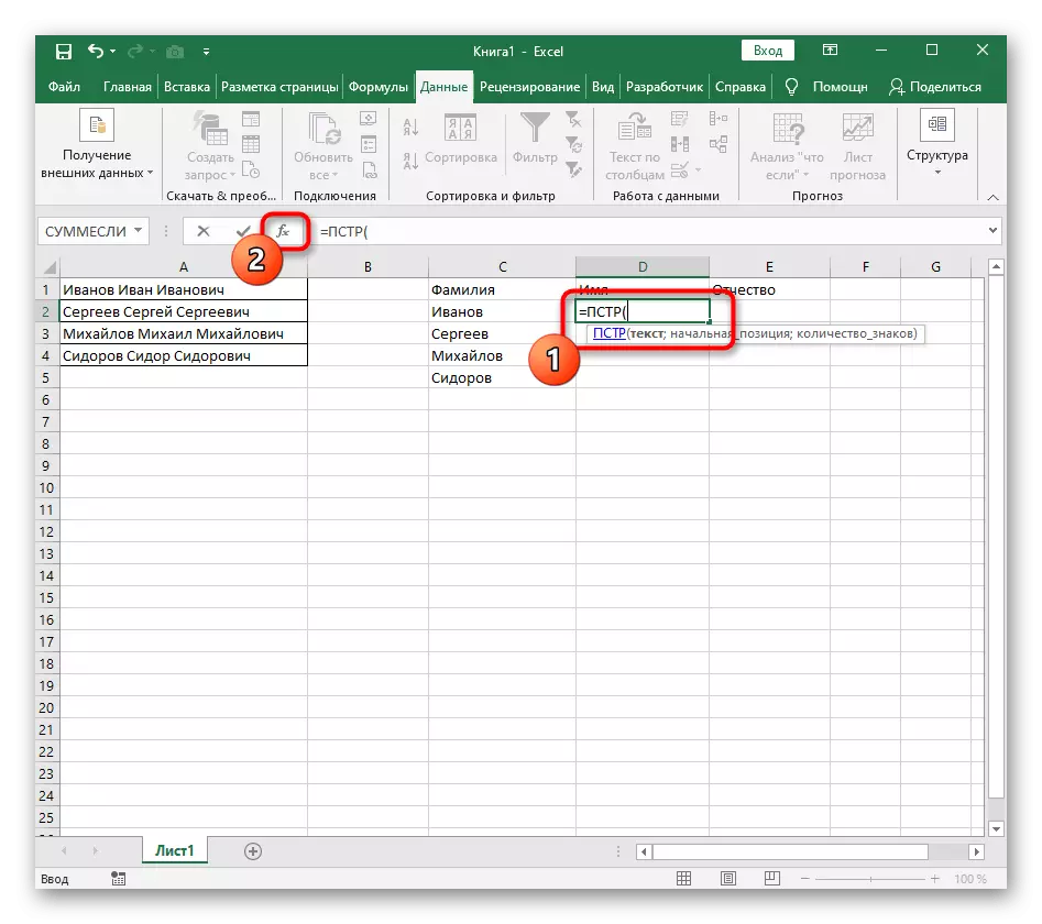
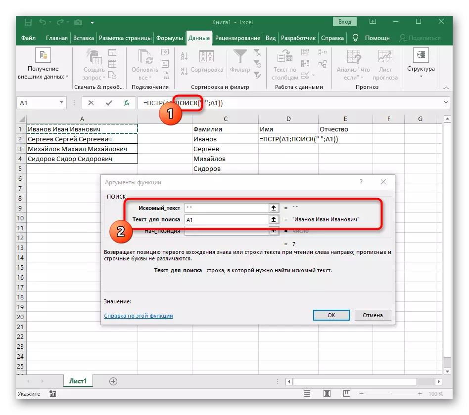
1. In this case, the main formula will be = PST (- write it in this form, and then go to the argument settings window.



2. This formula will search for the desired string in the text, which is chosen by the cell with an inscription for separation.



3. The initial position of the line will have to be determined using the already familiar auxiliary formula search ().



4. Creating and moving towards it, fill in the same way as it was shown in the previous step. As a desired text, use the separator, and specify the cell as text to search.



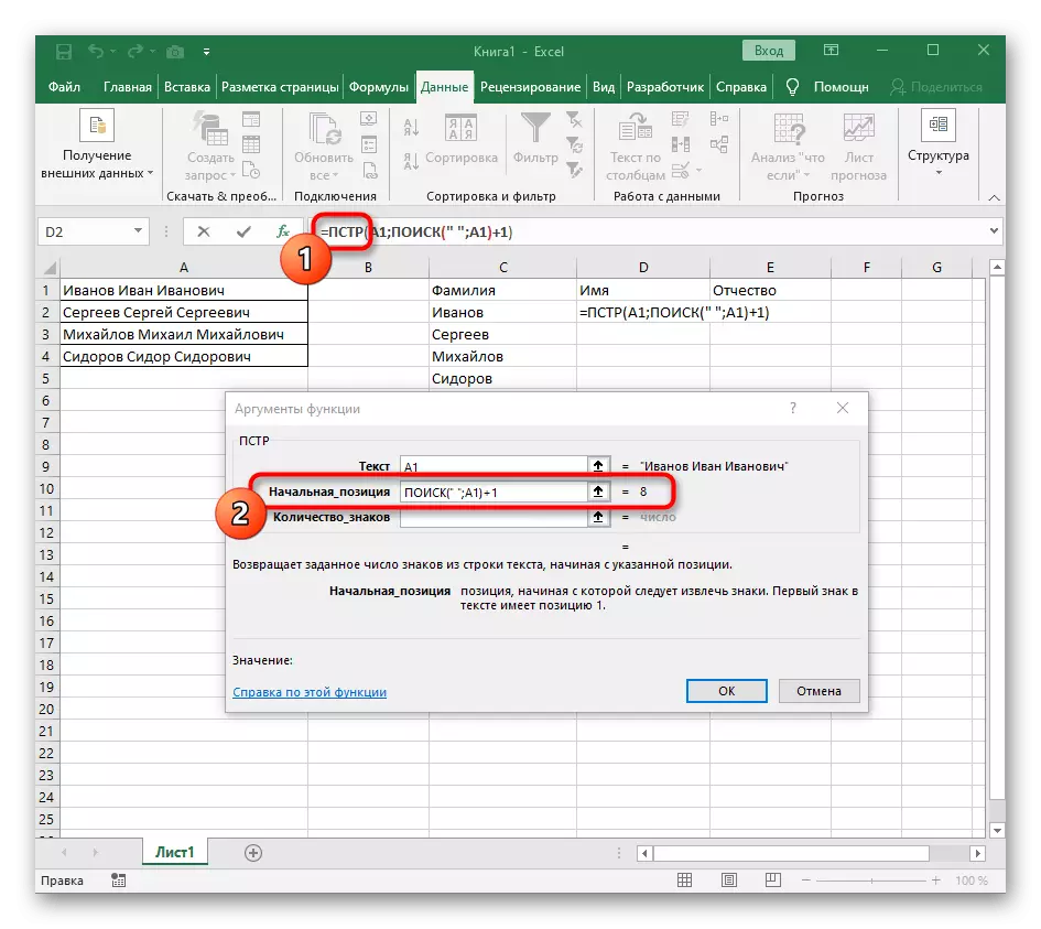
5. Return to the previous formula, where add to the "Search" function +1 at the end to start an account from the next character after the space found.



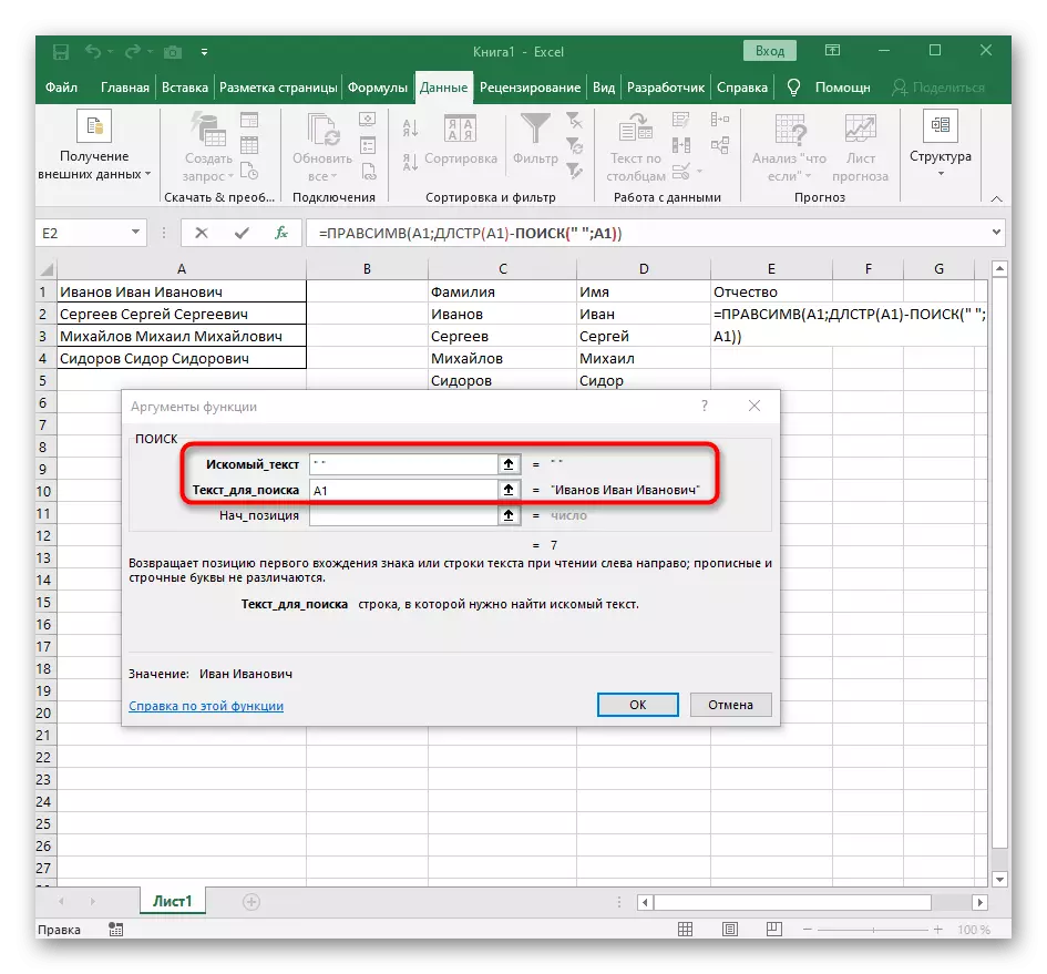
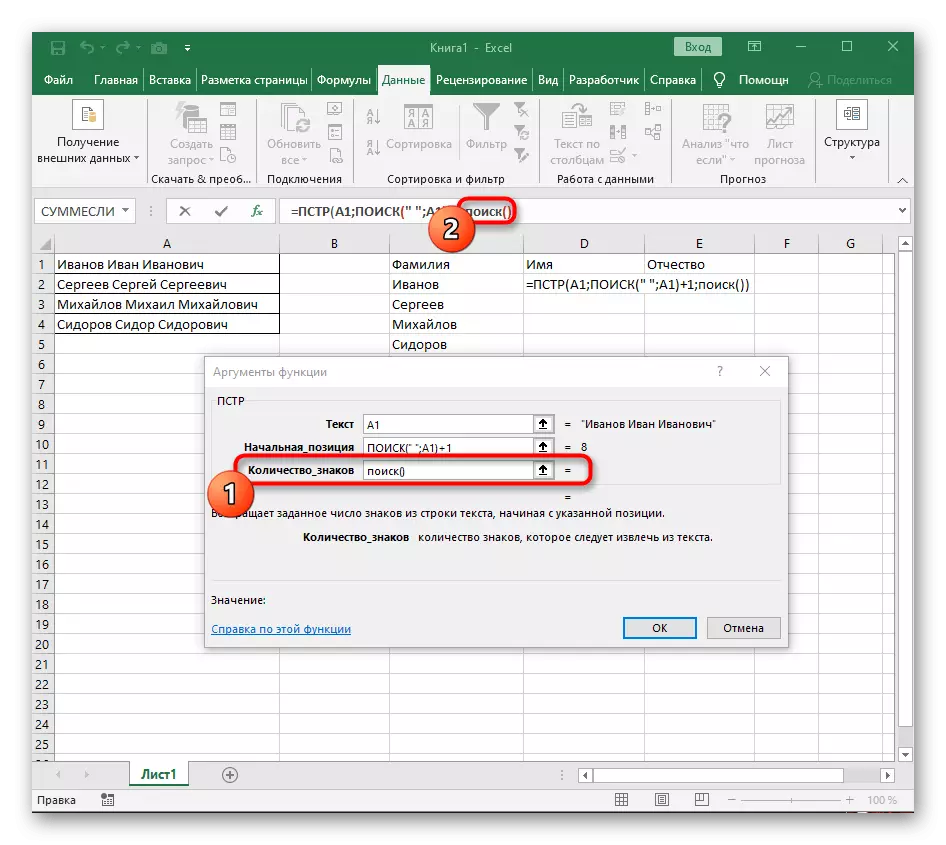
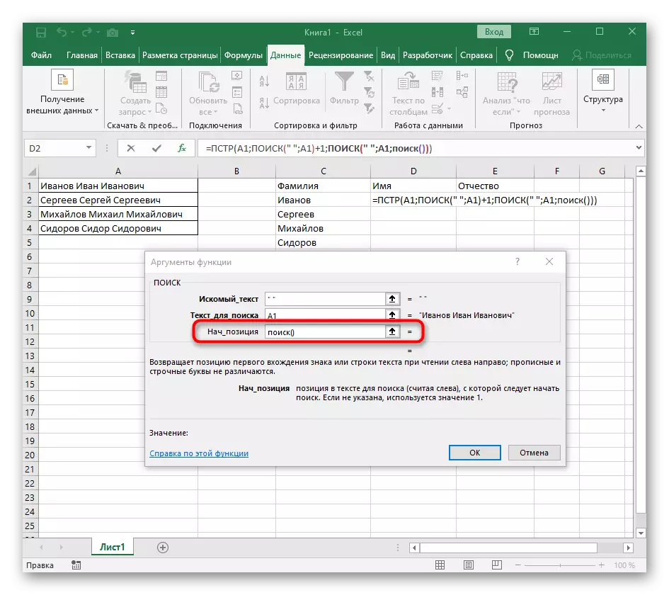
6. Now the formula can already start searching the line from the first character name, but it still does not know where to finish it, therefore, in the field "Quantity_names" again, write the search formula ().



7. Go to its arguments and fill them in the already familiar form.



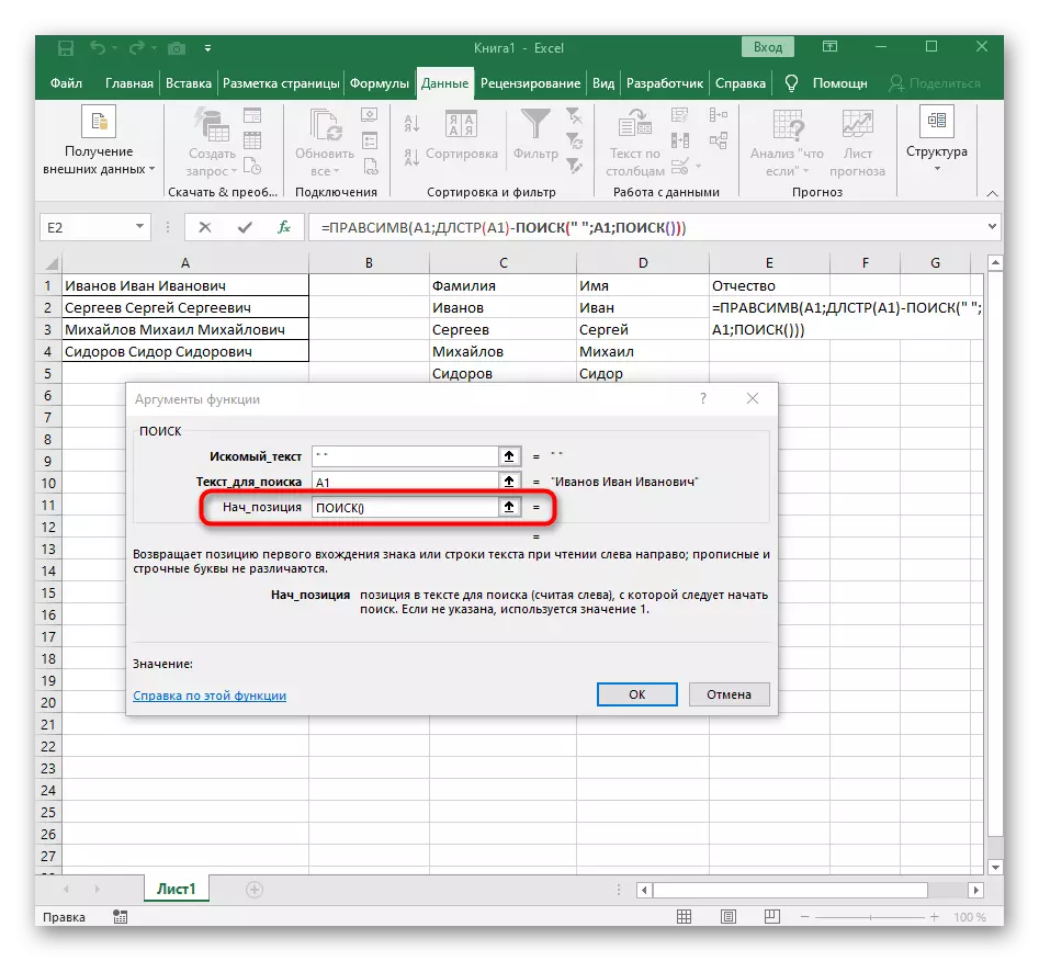
8. Previously, we did not consider the initial position of this function, but now it is necessary to enter the search (), since this formula should not find a first gap, but the second.



9. Go to the created function and fill it in the same way.



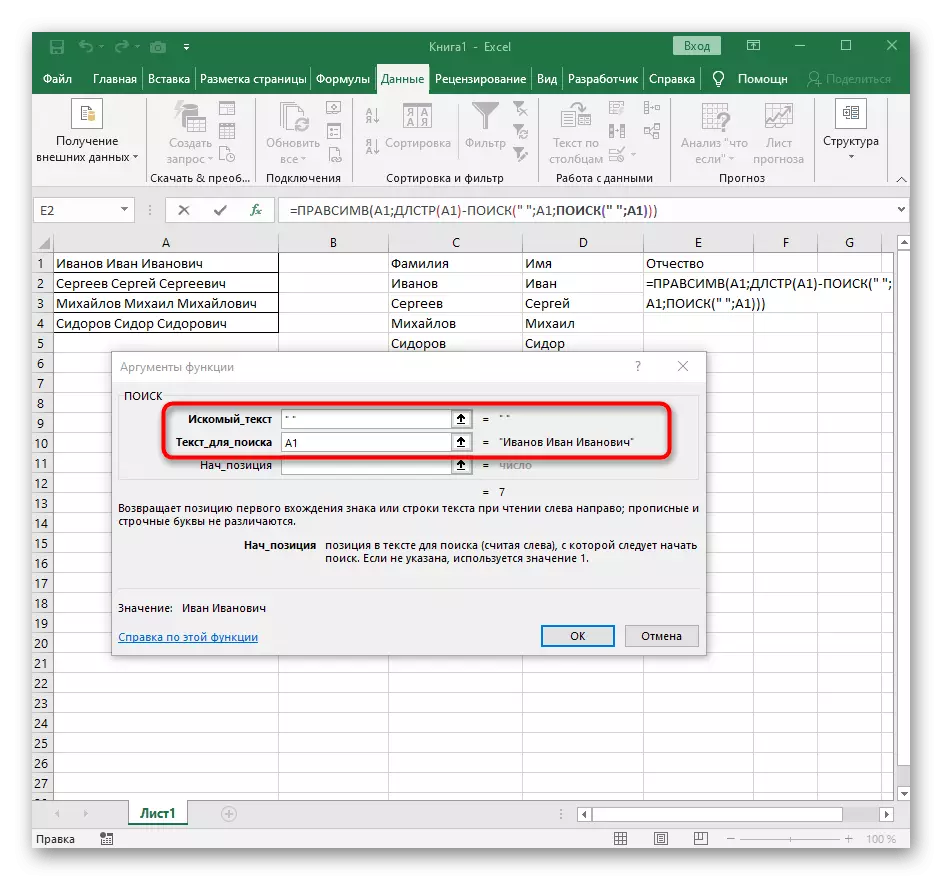
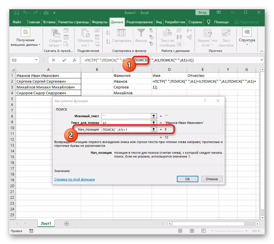
10. Return to the first "search" and add in the "Nach_POSITION" +1 at the end, because it does not need a space for searching the line, but the next character.



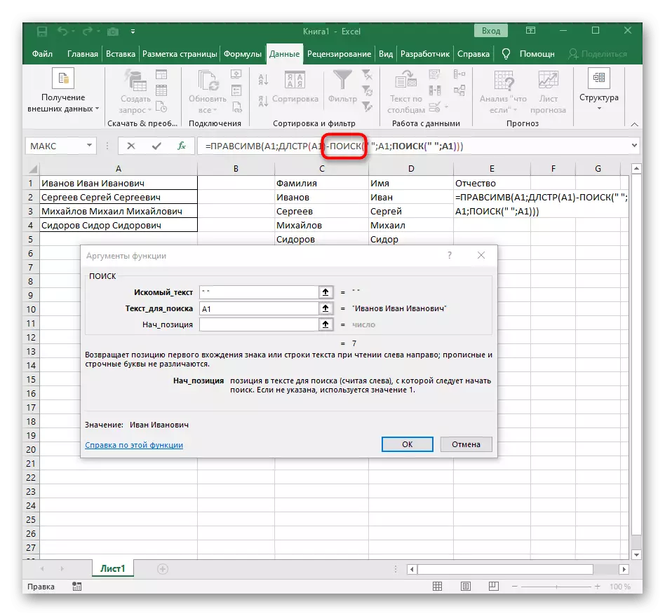
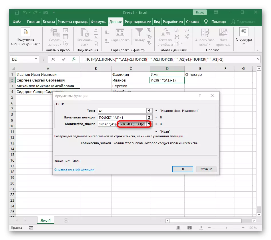
11. Click on the root = PST and put the cursor at the end of the line "Number_names".



12. Extract the expression of the expression (""; A1) -1 to complete the calculations of spaces.



13. Return to the table, stretch the formula and make sure that the words are displayed correctly.

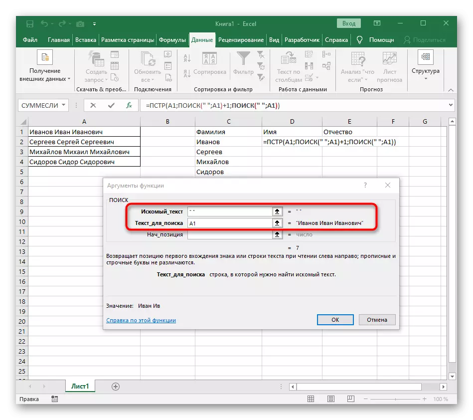
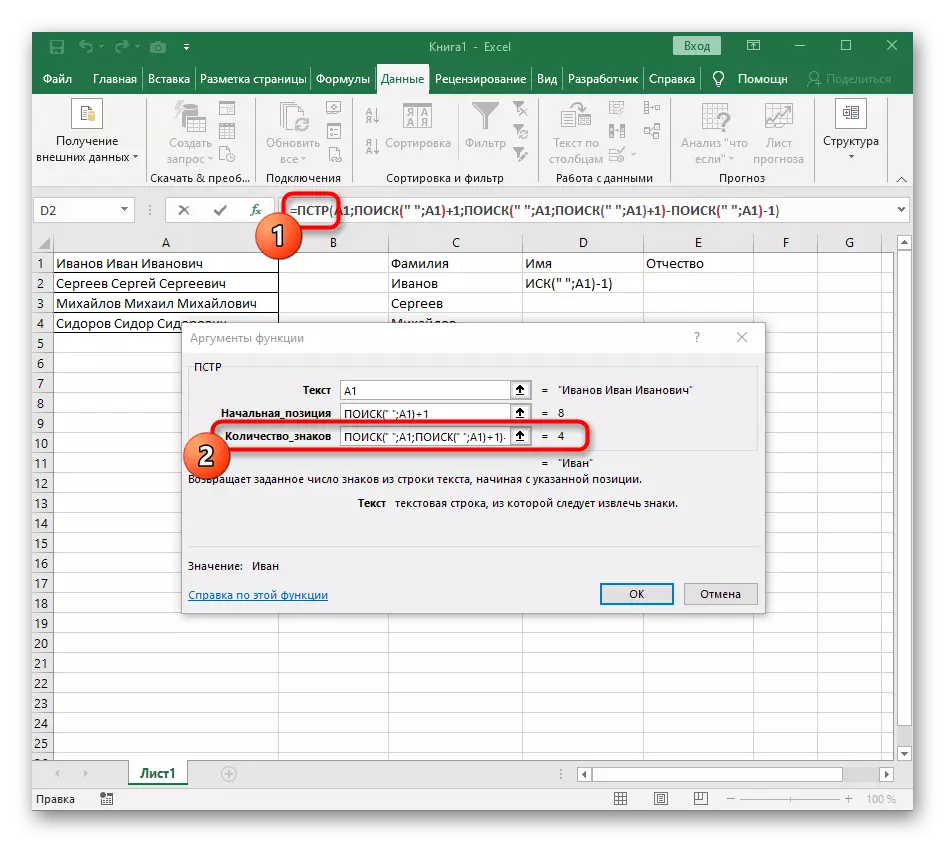
The formula turned out big, and not all users understand exactly how it works. The fact is that to search for the line I had to use several functions that determine the initial and final positions of spaces, and then one symbol took away from them so that as a result, these most gaps were displayed. As a result, the formula is this: = PSTr (A1; search (""; A1) +1; search (""; A1; search (""; A1) +1) -Poisk (""; A1) -1). Use it as an example, replacing the cell number with the text.

Step 3: Separation of the third word

The last step of our instruction implies the division of the third word, which looks about the same way as it happened with the first, but the general formula changes slightly.

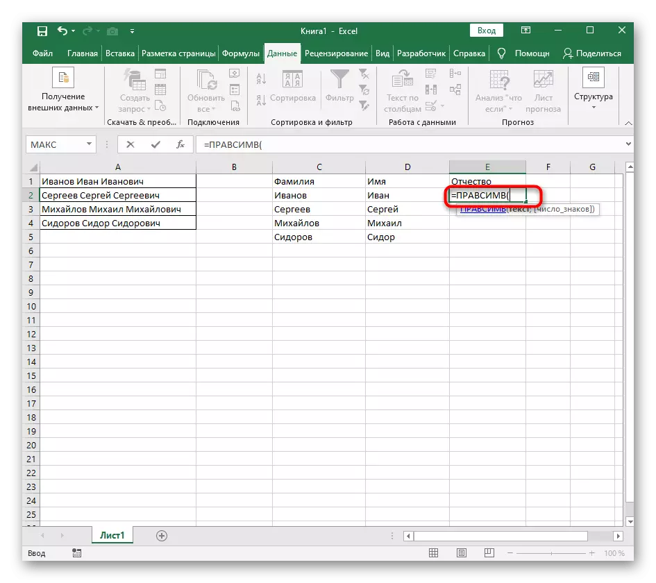
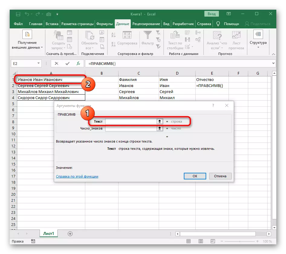
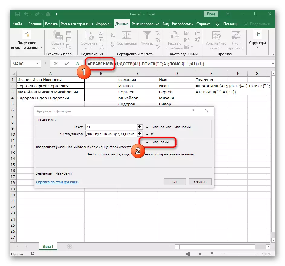
1. In an empty cell, for the location of the future text, write = Rashesimv (and go to the arguments of this function.



2. As a text, specify a cell with an inscription for separation.



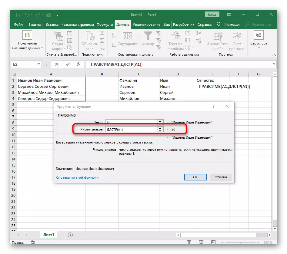
3. This time auxiliary function for finding a word is called DLSTR (A1), where A1 is the same cell with the text. This feature determines the number of characters in the text, and we will remain allocate only suitable.



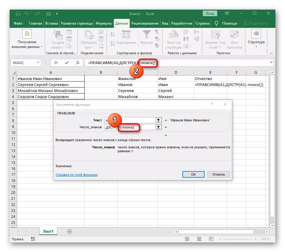
4. To do this, add -Poisk () and go to edit this formula.



5. Enter the already familiar structure to search for the first separator in the string.



6. Add another search for the starting position ().



7. Specify it the same structure.



8. Return to the previous search formula.



9. Add +1 to its initial position.



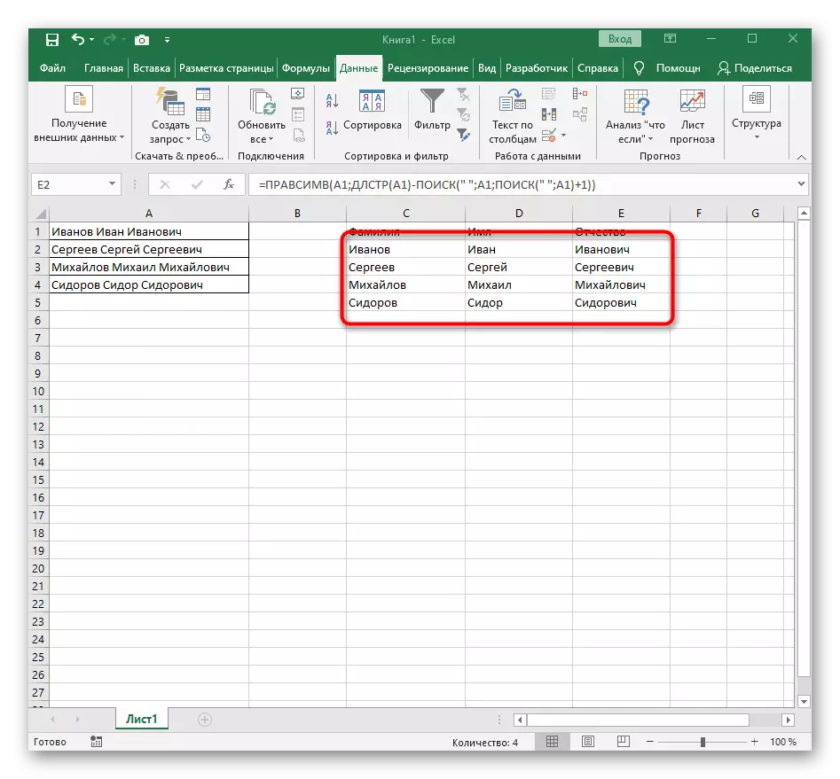
10. Navigate to the root of formula Rascessv and make sure that the result is displayed correctly, and then confirm the changes. The complete formula in this case looks like = Pracemir (A1; DLSTR (A1) -Poisk (""; A1; search (""; A1) +1)).



11. As a result, in the next screenshot you see that all three words are separated correctly and are in their columns. For this, it was necessary to use a variety of formulas and auxiliary functions, but it allows you to dynamically expand the table and do not worry that every time you have to share the text again. If necessary, simply expand the formula by moving it down so that the following cells are automatically affected.