
After building diagrams in the Microsoft Excel program, the default axes remain unsigned. Of course, it greatly makes it difficult to understand the contents of the diagram. In this case, the question of displaying the name on the axes becomes relevant. Let's figure out how to sign the axis of the diagram in the Microsoft Excel program, and how to assign named it.
Name of vertical axis
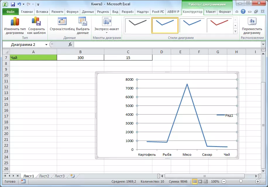
So, we have a ready diagram in which you need to give the names of the axes.
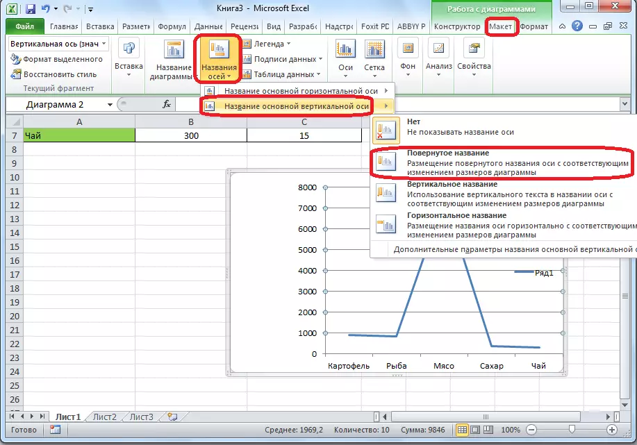
In order to assign the name of the vertical axis of the diagram, go to the "Layout" tab of the Master of Works with charts on the Microsoft Excel ribbon. Click on the "axis name" button. We choose, the item "name of the main vertical axis". Then, choose exactly where the name will be located.
There are three options for the name:
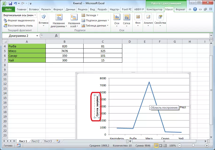
- Rotated;
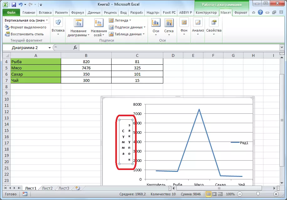
- Vertical;
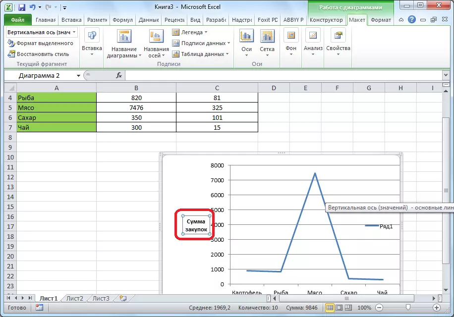
- Horizontal.
We choose, let's say turned title.
The default inscription appears, which is called the "axis name".
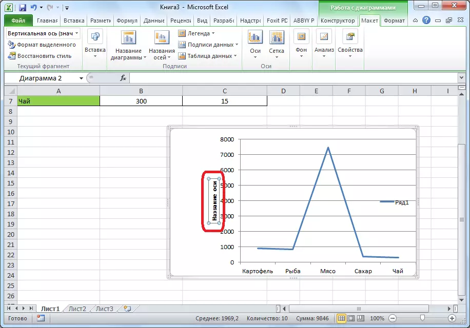
Just click on it, and we rename the name that suits this axis by the context.
If you choose a vertical placement of the name, the type of inscription will be the following as presented below.
With horizontal placement, the inscription will be deployed as follows.
The name of the horizontal axis
Almost in a similar way, the name of the horizontal axis is assigned.
Click on the button "Name axes", but this time I choose the item "name of the main horizontal axis". There is only one accommodation option - "under the axis". Choosing it.
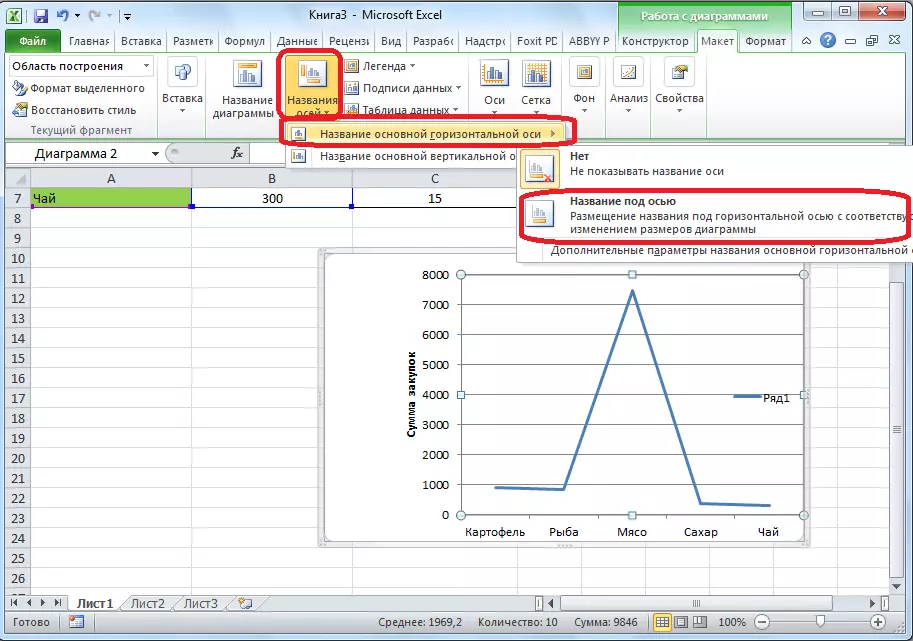
As last time, just click on the name, and change the name to the one that we consider it necessary.
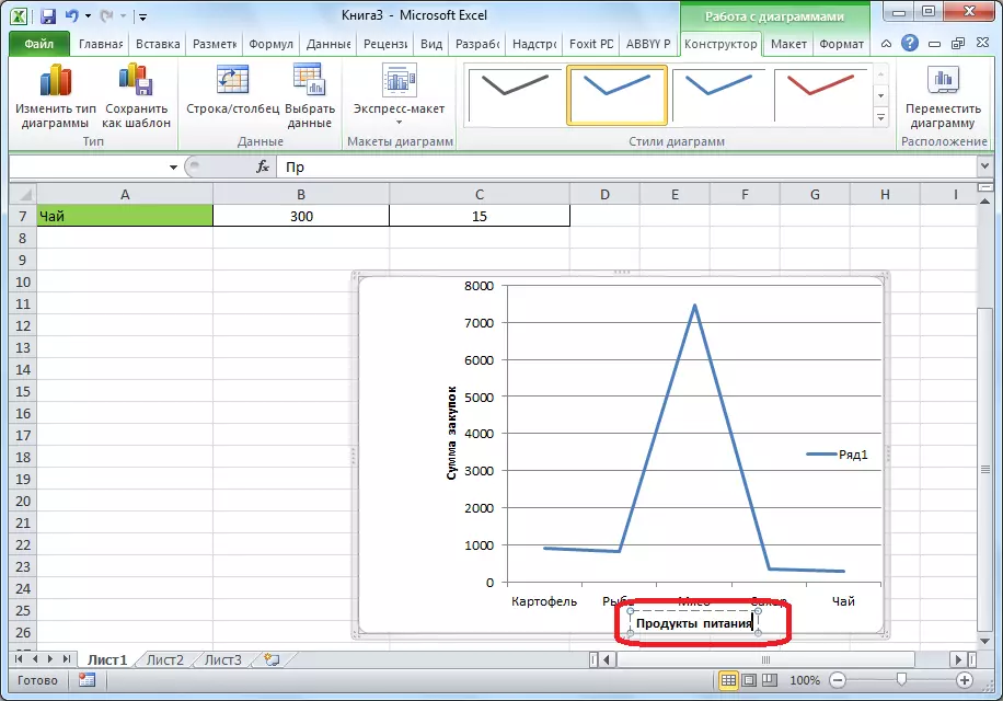
Thus, the names of both axes are assigned.
Change horizontal signature
In addition to the name, the axis has signatures, that is, the names of the values of each division. You can make some changes with them.
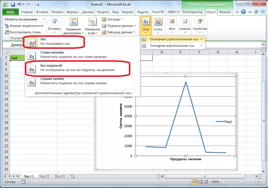
In order to change the type of signature of the horizontal axis, click on the "axis" button, and select the value "Main horizontal axis" there. By default, the signature is placed on the left right. But by clicking on the items "No" or "no signatures", you can generally disable the display of the horizontal signature.
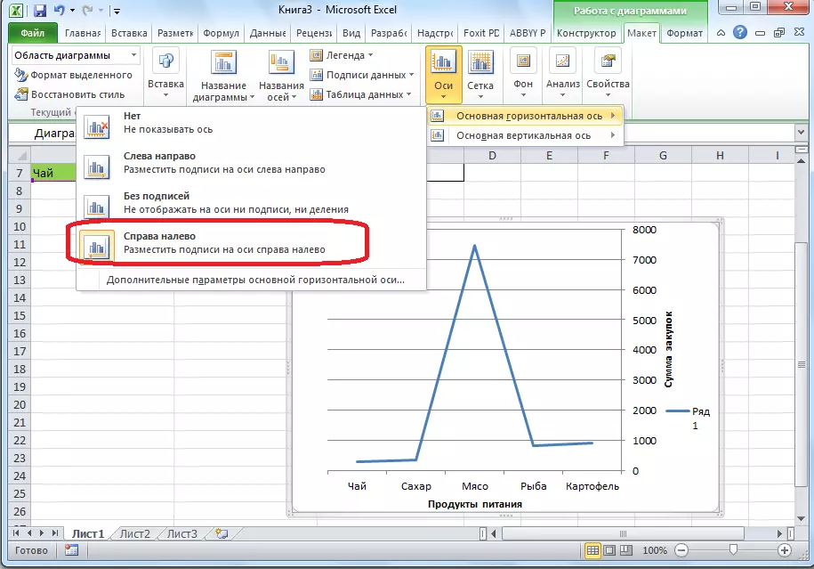
And after clicking on the item "right to left", the signature changes its direction.
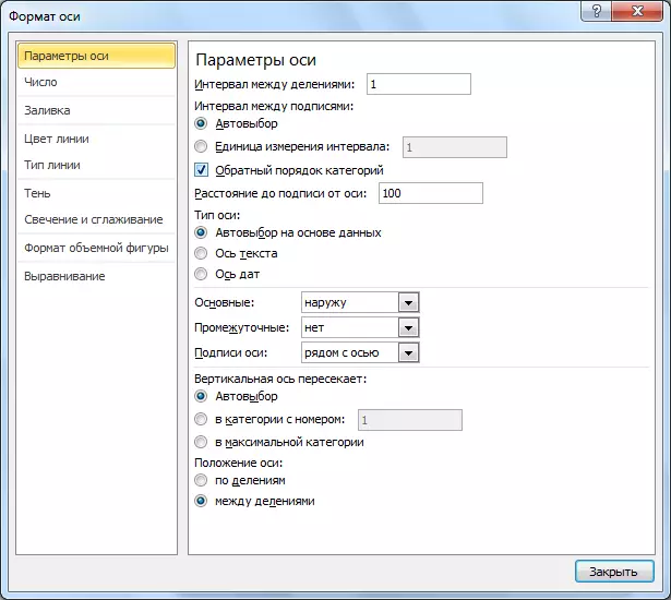
Furthermore, you can click on the item "More Options ... main horizontal axis".
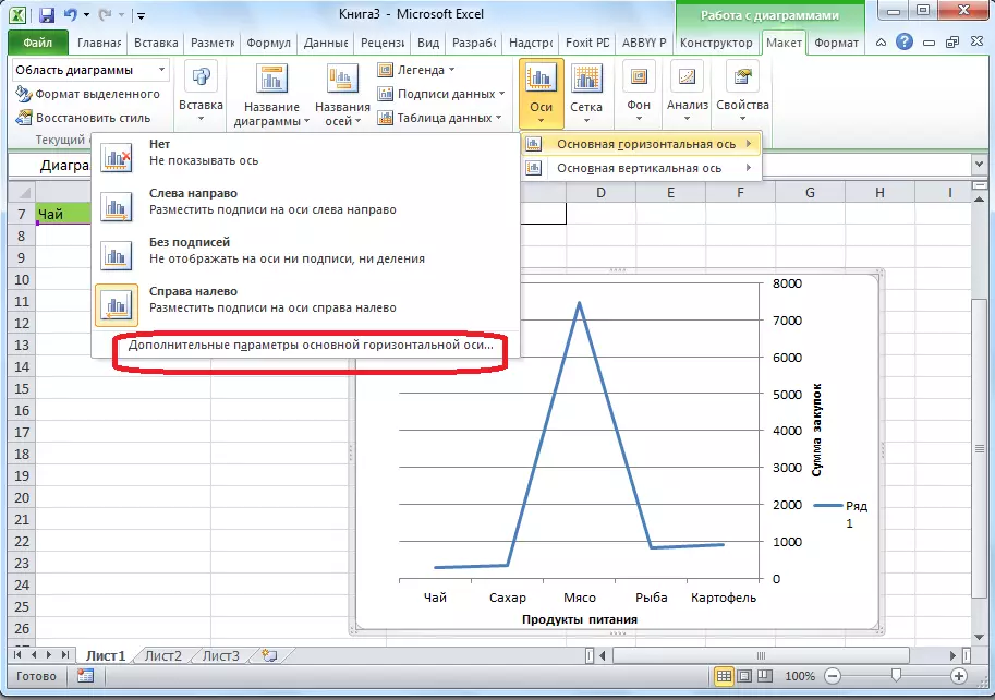
After that, a window opens, which offers a range of axis display settings: mark interval, the line color, the signature data format (numeric, money, text, etc.), line type, alignment, and more.
The change in vertical signature
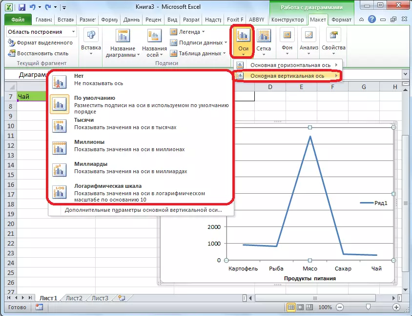
To change the vertical signature, click on the button "Axis", and then go under the name "The main vertical axis." As you can see, in this case, it seems to us more options in selecting accommodation signature on the axis. You can even skip the axis, and you can choose one of four options for displaying numbers:
- in thousands;
- in millions;
- in billions;
- a logarithmic scale.
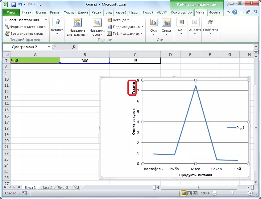
How can we demonstrate the chart below, then select an item, and change accordingly the scale.
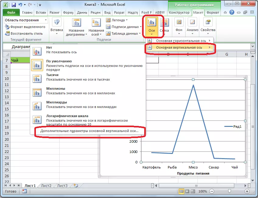
In addition, here you can select "Advanced Settings main vertical axis ...". They are similar to the corresponding item to the horizontal axis.
As you can see, the inclusion of the names and signatures of the axes in Microsoft Excel process is not particularly difficult, and, in general, intuitive. But, still it is easier to understand, having at hand a detailed action guide. Thus, you can save a lot of time researching these opportunities.