

For convenience of working with a large data array in tables, they are constantly necessary to organize according to a specific criterion. In addition, to fulfill specific purposes, sometimes the entire data array is not needed, but only individual lines. Therefore, in order not to be confused in a huge amount of information, the rational solution will be arranged data, and filter from other results. Let's find out how sorting and filtering data in Microsoft Excel is performed.
Simple data sorting
Sorting is one of the most convenient tools when working in Microsoft Excel. Using it, you can position the lines of the table in alphabetical order, according to data that are located in column cells.
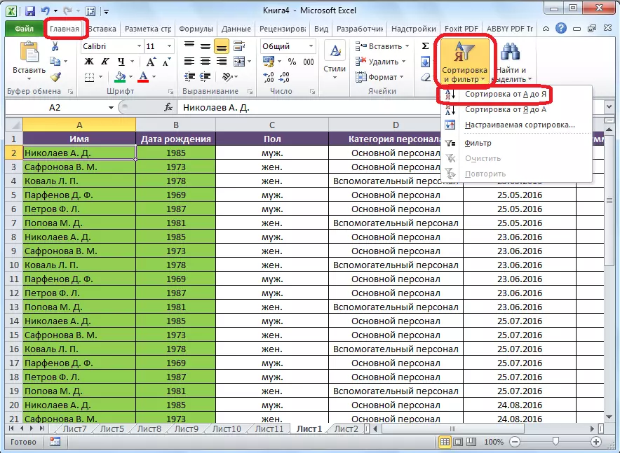
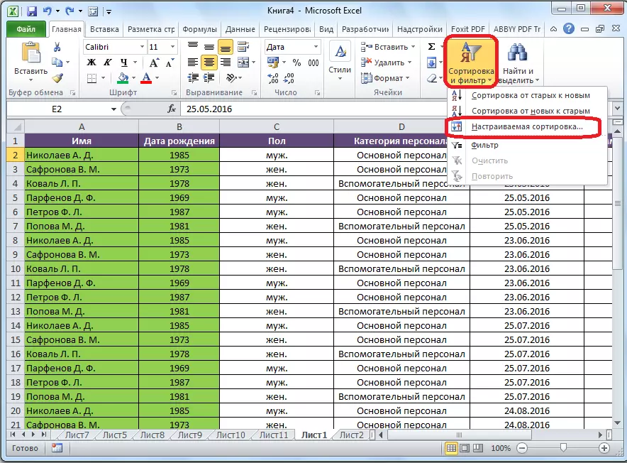
Data sorting in the Microsoft Excel program can be performed using the "Sort and Filter" button, which is posted in the Home tab on the tape in the Editing toolbar. But, before, we need to click on any cell of that column by which we are going to perform sorting.
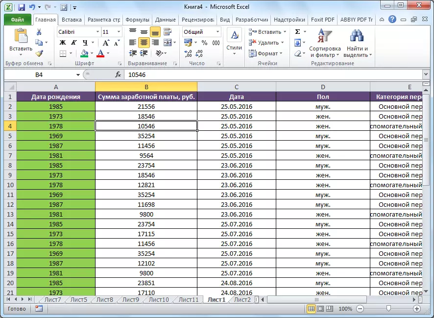
For example, in the table proposed below, it is necessary to sort the employees by the alphabet. We become in any cell of the "Name" column, and click on the "Sort and Filter" button. So that the names are arranged by alphabetically, choose the item "Sort from A to Z" from the list.
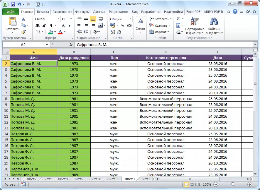
As you can see, all data in the table is located, according to the alphabetic list of surnames.

In order to sort in the reverse order, in the same menu, select the sort button from I up to A ".
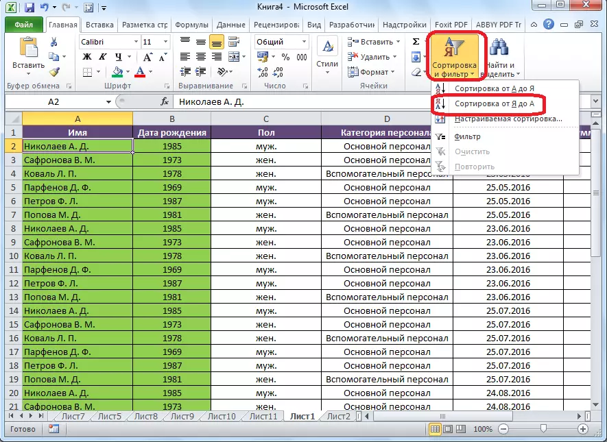
The list is rebuilt in the reverse order.
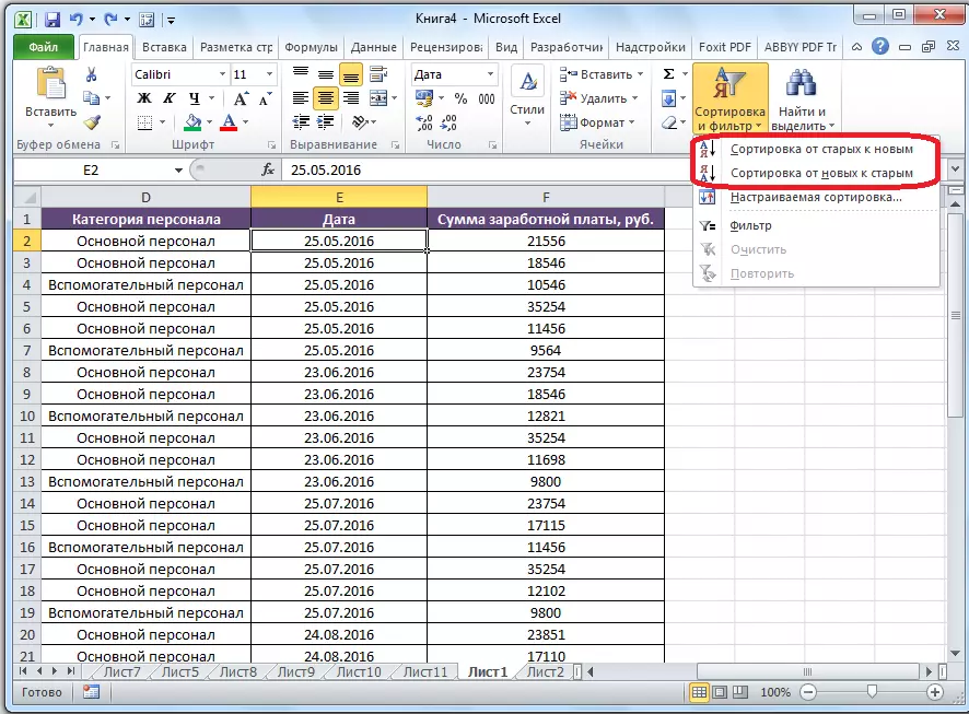
It should be noted that a similar type of sorting is indicated only with text data format. For example, with a numeric format, the sorting "from the minimum to the maximum" (and, on the contrary), and when the date format is "from the old to the new" (and, on the contrary).
Customizable sorting
But, as we see, with the specified types of sorting by one value, the data containing the names of the same person is built inside the range in an arbitrary order.
And what to do if we want to sort the names according to the alphabet, but for example, when you match the name so that the data is located by date? For this, as well as to use some other features, everything in the same menu "Sort and filter", we need to go to the item "Customizable Sorting ...".
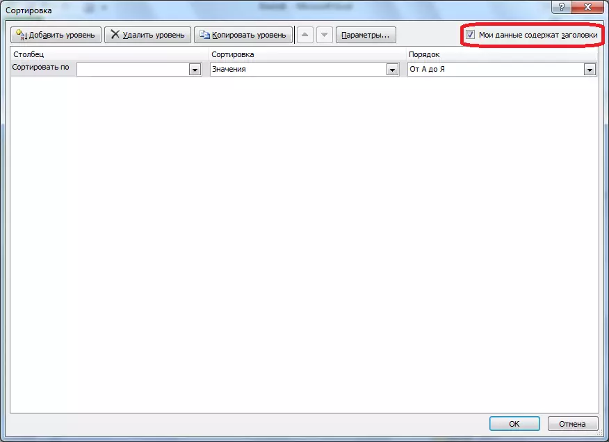
After that, the sorting settings window opens. If there are headlines in your table, please note that in this window it is necessary to stood a check mark near the "My data contains" parameter.
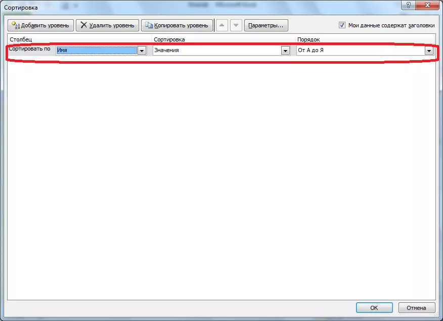
In the "Column" field, specify the name of the column by which sorting will be performed. In our case, this is the "Name" column. In the "Sort" field, it is specified according to what kind of content the content will be sorted. There are four options:
- Values;
- Cell color;
- Font color;
- Cell icon.
But, in the overwhelming majority, the item "Values" is used. He is set by default. In our case, we will also use this item.
In the column "order" we need to specify, in what order the data will be located: "From A to Z" or vice versa. Select the value "from A to Z."
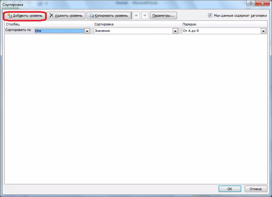
So, we set up the sorting one of the columns. In order to configure sorting on another column, click on the "Add Level" button.
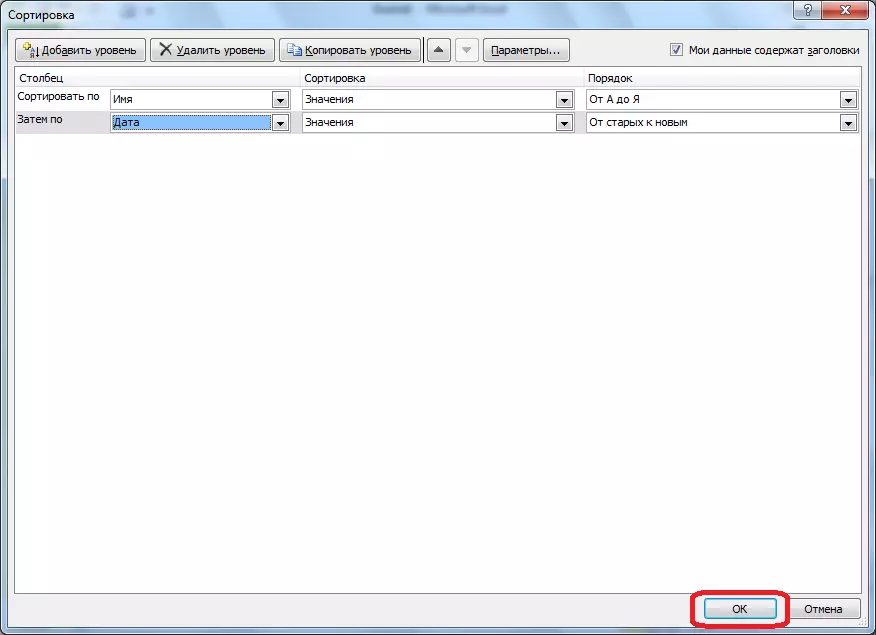
Another set of fields appears, which should be fill out for sorting through another column. In our case, according to the "date" column. Since the date of these cells is set to date, then in the "order" field we set the values not "from A to Z", but "from the old to new", or "from the new to the old".
In the same way, in this window you can configure, if necessary, and sorting over other columns in order of priority. When all settings are made, click on the "OK" button.
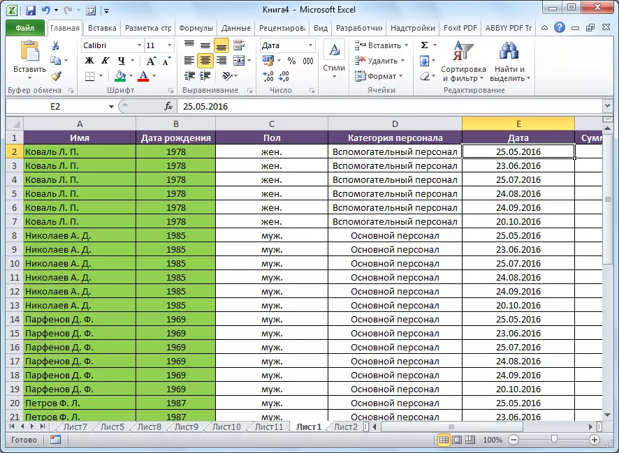
As you can see, now in our table all data sorted, first of all, by employee names, and then, by payout dates.
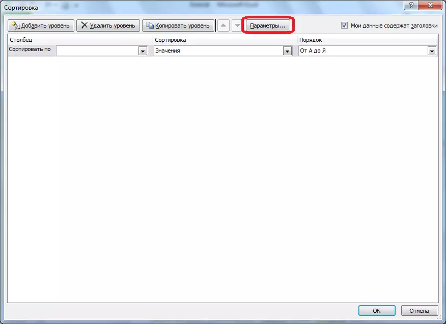
But, this is not all the possibilities of custom sorting. If desired, in this window, you can configure the sorting of non-columns, but by lines. To do this, click on the "Parameters" button.
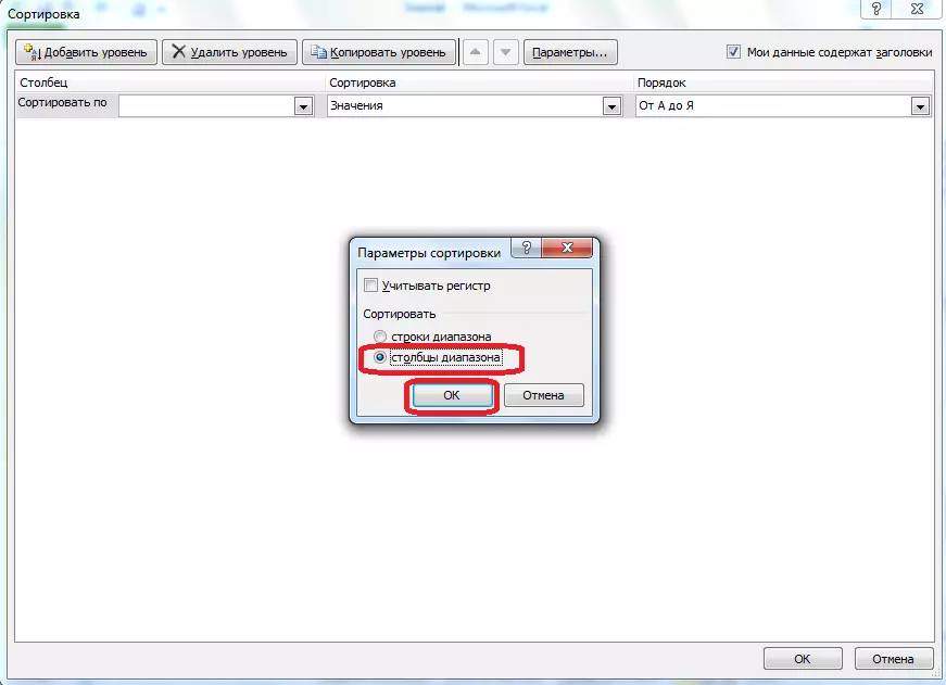
In the sorting parameters window that opens, we translate the switch from the "Row Row" position to the "range columns" position. Click on the "OK" button.
Now, by analogy with the previous example, you can inscribe data for sorting. Enter the data, and click on the "OK" button.

As we see, after that, the columns changed places, according to the parameters entered.
Of course, for our table, taken for example, the use of sorting with a change in the location of the column does not carry a special use, but for some other tables such a kind of sorting can be very relevant.
Filter
In addition, in Microsoft Excel, there is a data filter function. It allows you to leave visible only those data that you consider the necessary, and the rest hide. If necessary, hidden data can always be returned to the visible mode.
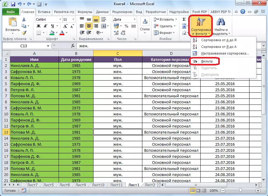
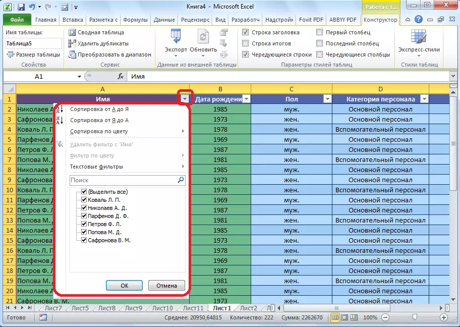
To use this feature, we become on any cell in the table (and preferably in the header), again we click on the "Sort and Filter" button in the Editing toolbox. But, this time in the menu that appears, select the "Filter" item. You can also instead of these actions simply press the CTRL + SHIFT + L key combination.

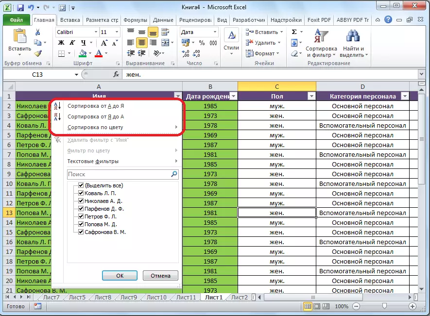
As we can see, the cells in the form of a square appeared in the cells with the name of all columns, in which the triangle is inverted down.
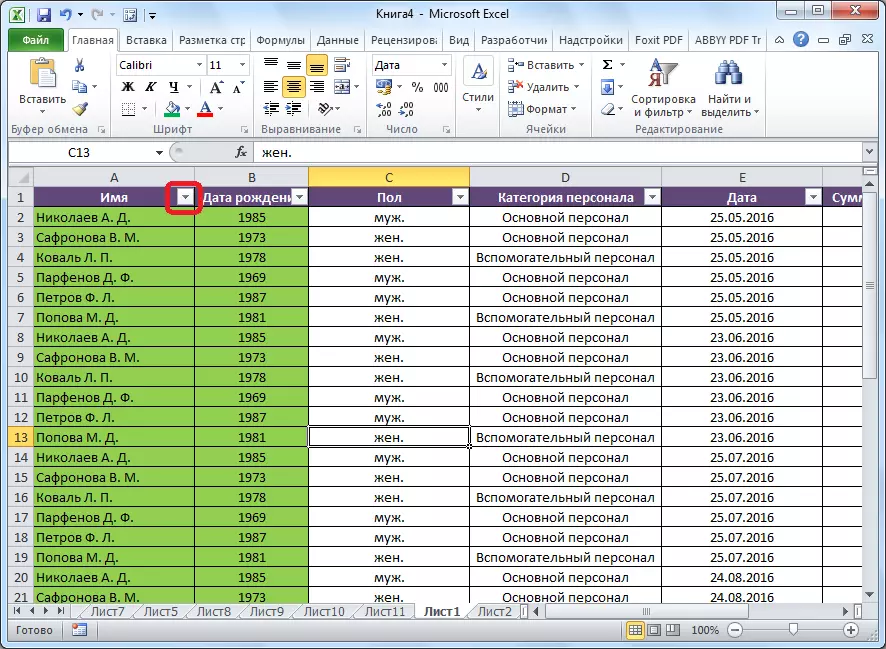
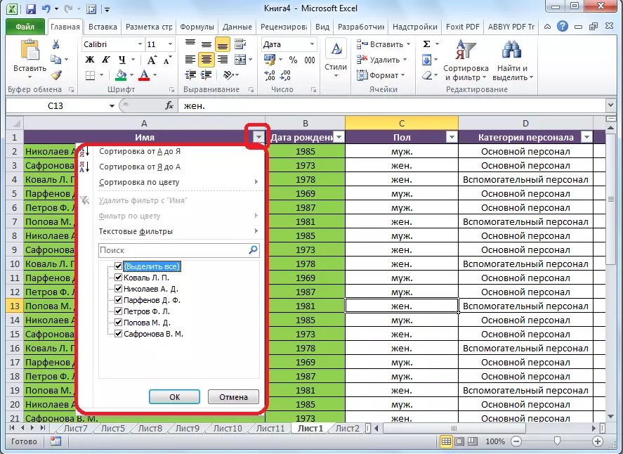
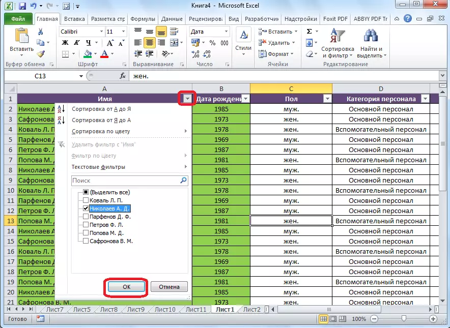
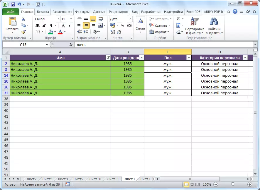
Click on this icon in the column, according to which we are going to filter. In our case, we decided to filter by name. For example, we need to leave the data only by the employee of Nikolaev. Therefore, shoot ticks from the names of all other workers.
When the procedure is made, click on the "OK" button.
As we can see, only strings with the name of the employee of Nikolaev remained in the table.
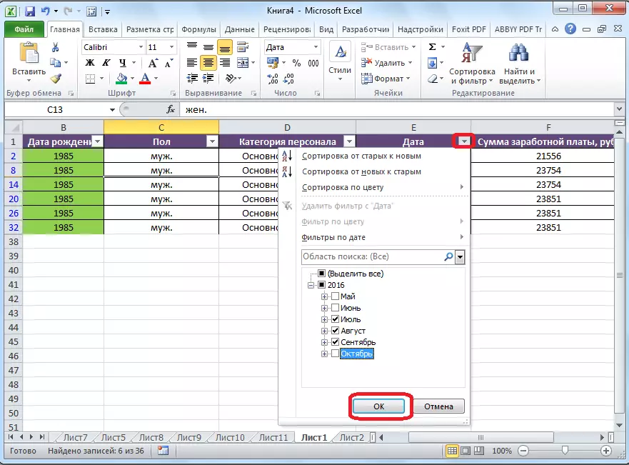
Complete the task, and we will only leave the table in the table that relate to Nikolaev for the III quarter of 2016. To do this, click on the icon in the Date Cell. In the list that opens, remove the checkboxes from the months "May", "June" and "October", as they do not belong to the third quarter, and click on the "OK" button.
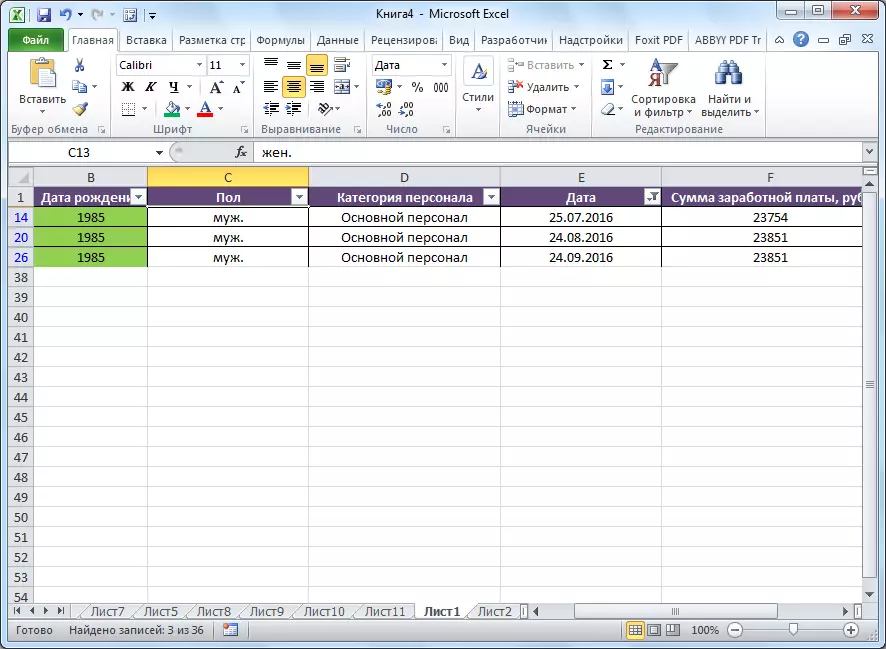
As you can see, only the data we need remained.
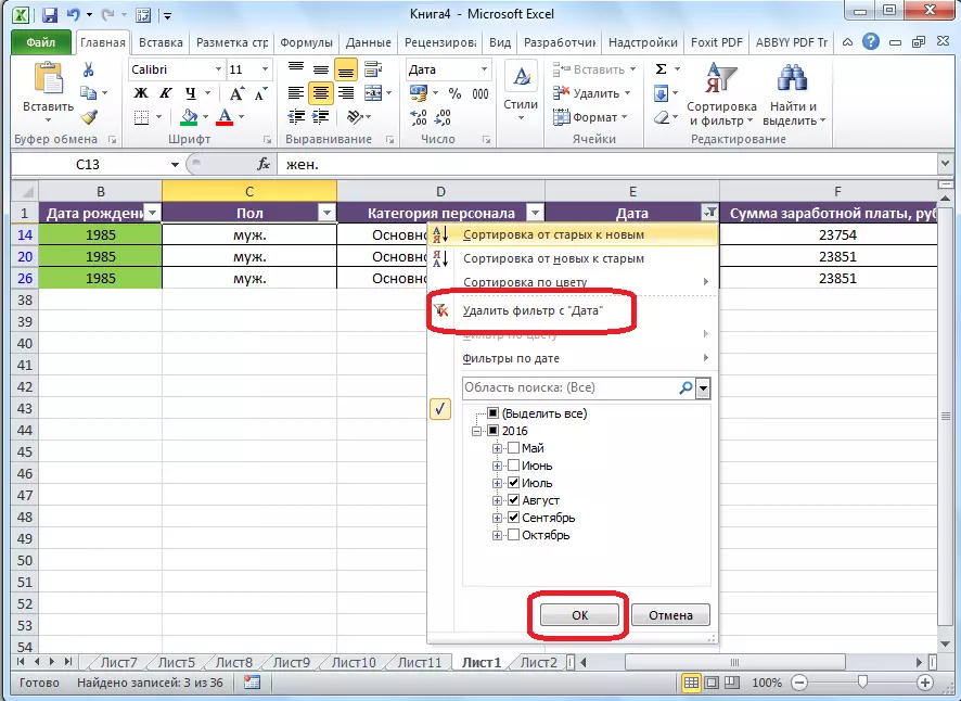
In order to remove the filter on a specific column, and show the hidden data, again, click on the icon located in the cell with the title of this column. In the open menu, click on "Delete Filter C ..." item.
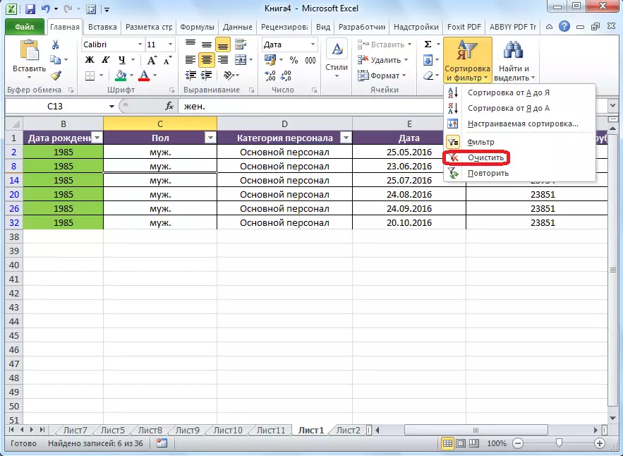
If you want to reset the filter as a whole on the table, then you need to click the "Sort and Filter" button on the tape, and select "Clear".
If you need to completely remove the filter, then, like when it starts, you should select the "Filter" item in the same menu, or type the keyboard key on the CTRL + SHIFT + L keyboard.
In addition, it should be noted that after we have turned on the "Filter" function, then when you click on the corresponding icon in the cells of the table caps, the sorting functions that we spoke above are available in the menu that appeared: "Sort from A to Z" , "Sort from me to a", and "sorting in color."
Lesson: how to use autofilter in Microsoft Excel
Smart Table
Sorting and filter can also be activated, turning the area of the data with which you work in the so-called "smart table".
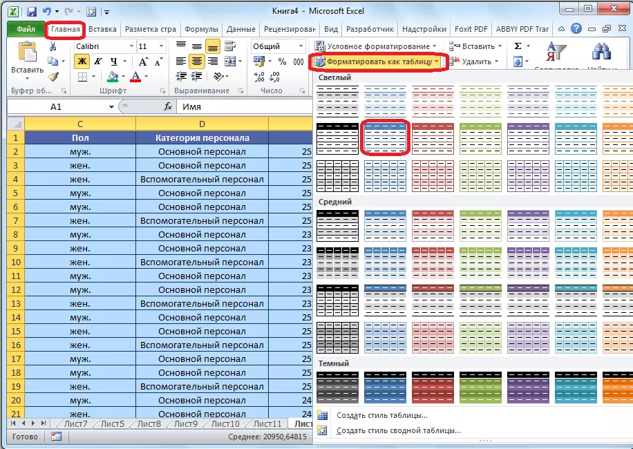
There are two ways to create a smart table. In order to take advantage of the first of them, allocate the entire area of the table, and, while in the "Home" tab, click on the button on the button "Format as a table". This button is in the "Styles" tool block.
Next, we choose one of the styles you like, in the list that opens. You will not affect the functionality of the table.
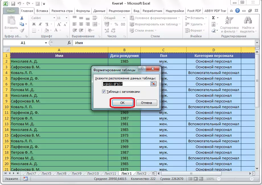
After that, a dialog box opens in which you can change the coordinates of the table. But if you previously allocated the area correctly, you don't need anything else. The main thing, note that the "Table with headlines" parameter stood a check mark. Next, just click on the "OK" button.
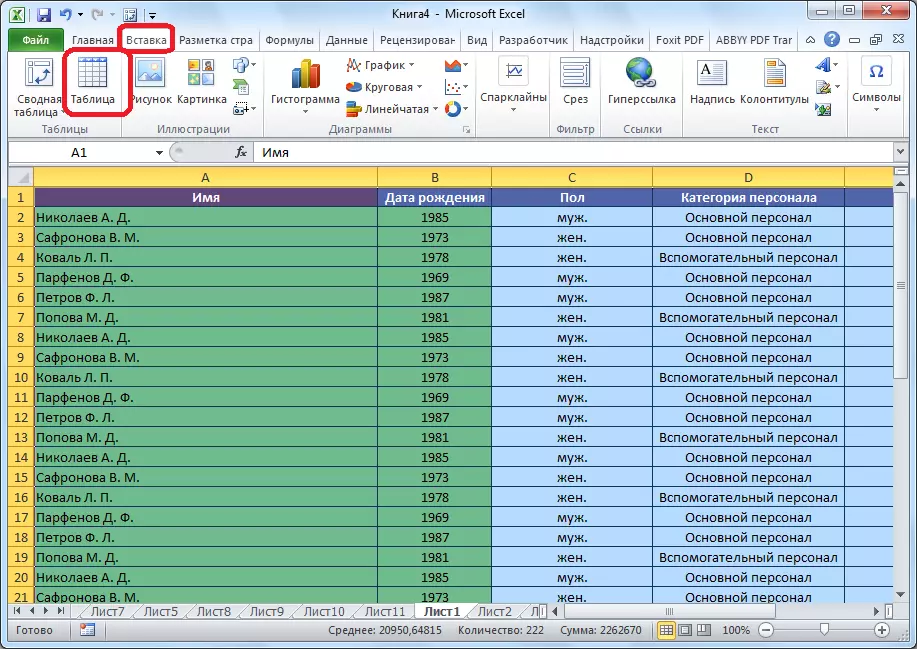
If you decide to take advantage of the second way, then you also need to highlight the entire area of the table, but this time go to the "Insert" tab. Being here, on the tape in the "Table Tools" block, you should click on the "Table" button.
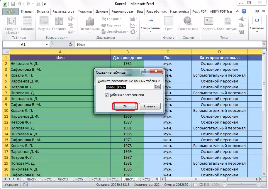
After that, as the last time, a window will open where the coordinates of the placement of the table will be corrected. Click on the "OK" button.
Regardless of how you use when creating a "smart table", we eventually get a table, in the cells of the caps of which the filters described by us have already been installed.
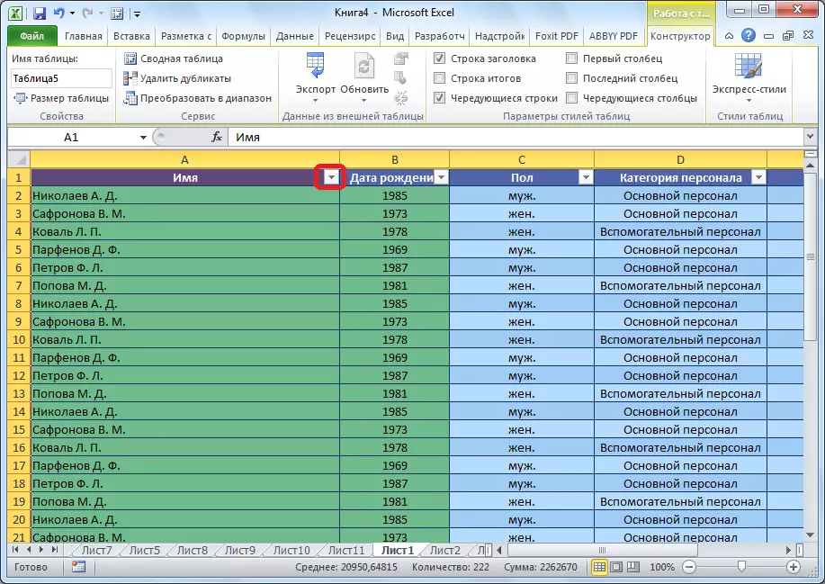
When you click on this icon, all the same functions will be available as when you start the filter with a standard way through the "Sort and Filter" button.
Lesson: How to create a table in Microsoft Excel
As you can see, sorting and filtering tools, with their proper use, can significantly facilitate users to work with tables. A particularly relevant issue of their use becomes in the event that a very large data array is recorded in the table.