

Looking at the dry digits of the tables, it is difficult at first glance to catch the overall picture they represent. But, in Microsoft Excel, there is a graphic visualization tool with which you can clearly submit the data contained in the tables. This allows you to more easily and quickly assimilate information. This tool is called conditional formatting. Let's figure out how to use conditional formatting in Microsoft Excel.
Simple conventional formatting options
In order to format a specific cell area, you need to highlight this area (most often column), and while in the Home tab, click on the Conditional Formatting button, which is located on the tape in the "Styles" tool block.
After that, the conditional formatting menu opens. Here are three main types of formatting:
- Histograms;
- Digital scales;
- Icons.

In order to carry out conditional formatting in the form of a histogram, select the column with data, and click on the appropriate menu item. As you can see, it seems to select several types of histograms with gradient and solid fill. Choose the one that, in your opinion, most matches the style and content of the table.

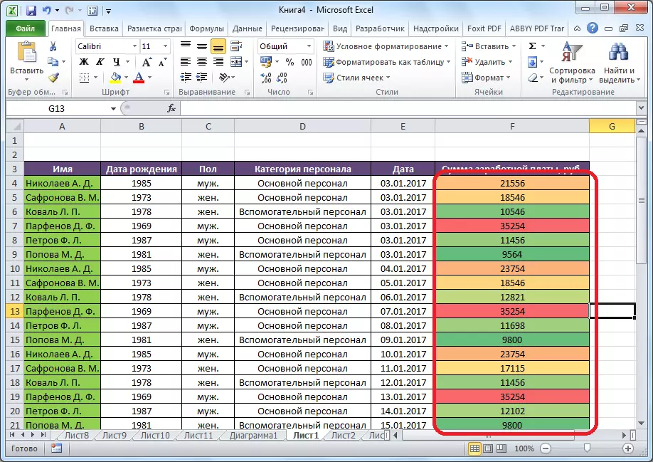
As you can see, the histograms appeared in the selected cells of the column. The greater the numeric value in the cells, the higher the histogram is longer. In addition, in the versions of Excel 2010, 2013 and 2016, there is the possibility of correctly displaying negative values in the histogram. But, in the 2007 version of this possibility.

When used instead of a histogram of the color scale, there is also the ability to choose various options for this tool. At the same time, as a rule, the greater the value is located in the cell, the time the color of the scale is richer.
The most interesting and complex tool among this set of formatting functions are icons. There are four main groups of icons: directions, figures, indicators and evaluations. Each user selected option involves the use of different icons when evaluating the contents of the cell. The entire selected area is scanned by Excel, and all cell values are separated into parts, according to the values specified in them. Green icons are used to the greatest quantities, the values of the middle range are yellow, and the magnitude, located in the smallest third - are marked with red icons.

When choosing a shooter, as icons, except for color design, used still signaling in the form of directions. So, the arrow rotated by the upward pointer is applied to large values, to the left - to the middle, down - to small. When using figures, the biggest values are marked, the triangle is medium, rhombus - small.

Rules for allocation of cells
By default, a rule is used, in which all cells of the dedicated fragment are designated in a specific color or a icon, according to the values located in them. But, using the menu, which we have already spoken above, you can apply other rules for the designation.
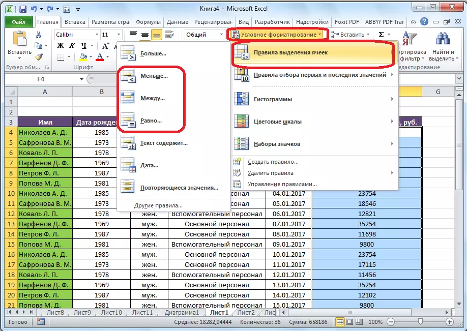
Click on the menu item "Rules for the allocation of cells". As you can see, there are seven basic rules:
- More;
- Smaller;
- Equals;
- Between;
- The date;
- Repeating values.

Consider the use of these actions on the examples. We highlight the range of cells, and click on the item "more ...".

A window opens in which you need to install, values more than what number will be stand out. It is done in the "Format cells that are more" field. By default, the average value of the range automatically fits here, but you can install any other, or specify the cell address containing this number. The last option is suitable for dynamic tables, the data in which is constantly changing, or for a cell, where the formula is applied. We for example set the value to 20,000.
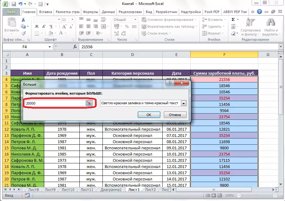
In the next field, you need to decide how cells will be released: light red fill and dark red (default); Yellow Pouring and Dark Yellow Text; Red text, etc. In addition, there is a custom format.

When you go to this item, a window opens in which you can edit the selection, practically, as if using various font options, fill, and boundaries.

After we have determined, with the values in the Settings window of the allocation rules, click on the "OK" button.

As you can see, cells are highlighted, according to the established rule.

By the same principle, values are allocated when applying the rules "less", "between" and "equal." Only in the first case, cells are highlighted less than the value set by you; in the second case, the interval of the numbers, the cells with which will be released; In the third case, a particular number is set, and cells only contain it will be distinguished.
The selection rule "Text contains" is mainly applied to text format cells. In the Rules Setup window, you should specify the word, part of the word, or a serial set of words, while finding which the corresponding cells will be allocated to the method you set.

The Date rule applies to cells that contain values in the date format. At the same time, in the settings you can set the selection of cells by the time when an event occurred: today, yesterday, tomorrow, for the last 7 days, etc.

Applying the "Repeating Values" rule, you can adjust the selection of cells, according to the correspondence of these data placed in them, one of the criteria: repeated data or unique.

The rules for the selection of the first and recent values
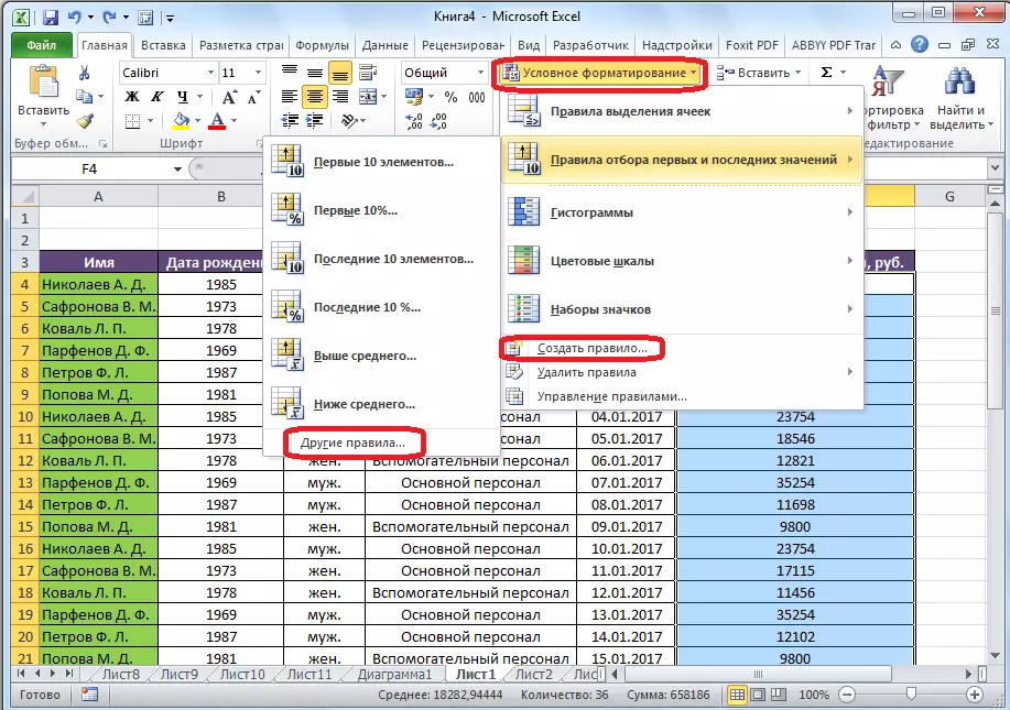
In addition, in the conditional formatting menu, there is another interesting point - "The rules for the selection of the first and last values." Here you can set the allocation of only the largest or smallest values in the range of cells. At the same time, the selection can be used, both for ordinal values and percentage. The following selection criteria exist, which are specified in the respective menu items:
- The first 10 elements;
- The first 10%;
- The last 10 elements;
- Last 10%;
- Above the average;
- Below the average.

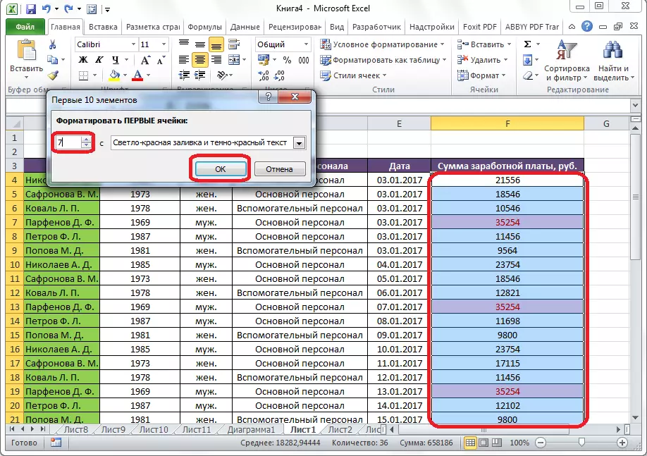
But after you clicked on the relevant item, you can change the rules slightly. A window opens, which uses the type of selection, as well as, if desired, you can install another selection limit. For example, we, by clicking on the "first 10 elements" item, in the window that opens, the number 10 to "format the first cells" is replaced in the "Format" field. Thus, after pressing the "OK" button, not 10 largest values, but Only 7.
Creation of rules
Above, we talked about the rules that are already installed in the Excel program, and the user can simply choose any of them. But, in addition, if desired, the user can create its own rules.
To do this, you need to click in any subsection of the conditional formatting menu to the item "Other Rules ..." located at the very bottom of the list. " Or click on the "Create Rule ..." item, which is located at the bottom of the main conditional formatting menu.
A window opens where you need to choose one of the six types of rules:
- Format all cells on the basis of their values;
- Format only cells that contain;
- Format only the first and last values;
- Format only values that are above or below average;
- Format only unique or repetitive values;
- Use the formula to determine the formatable cells.
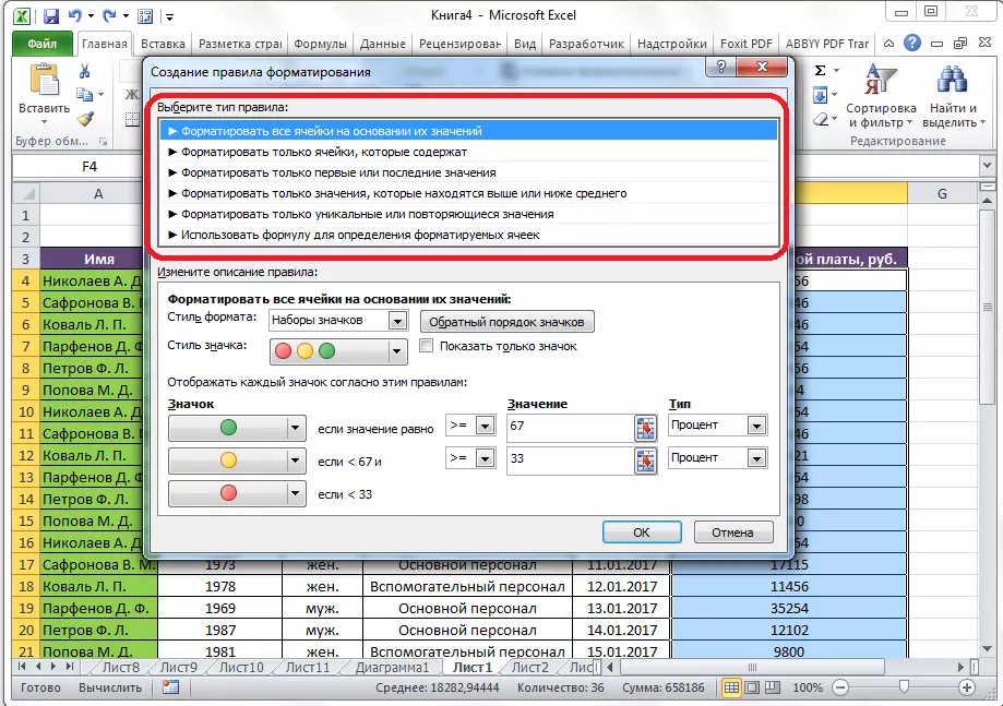
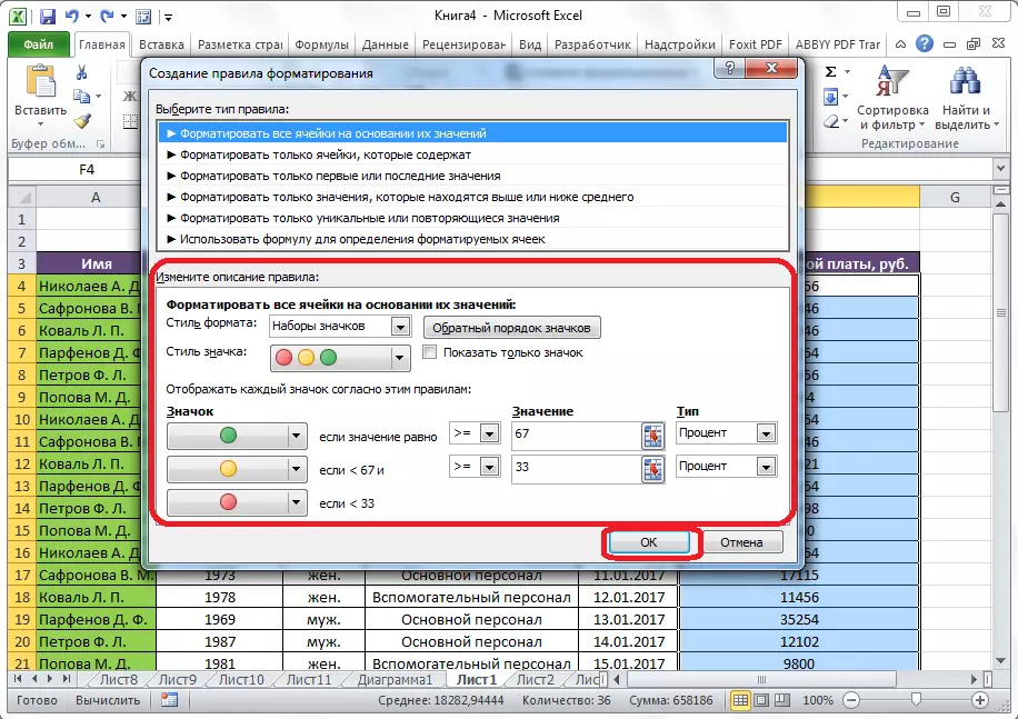
According to the selected rules type, at the bottom of the window, you need to configure the change in the description of the rules, setting the values, intervals and other values that we have already spoken below. Only in this case, the installation of these values will be more flexible. Immediately, with the help of changing the font, borders and fillings, exactly how to look like. After all the settings are made, you need to click on the "OK" button to save the changes made.
Rules Management
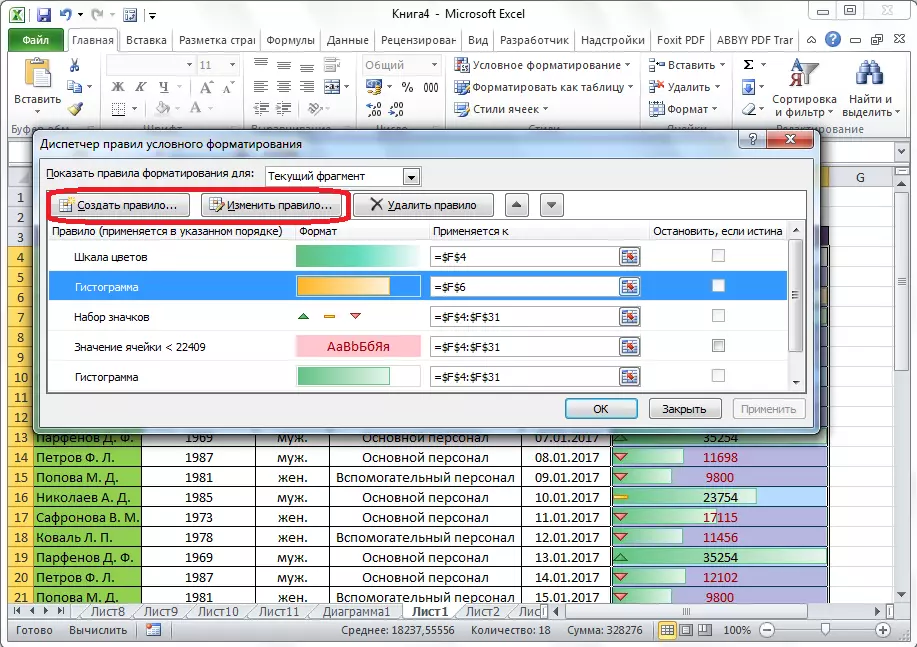
In Excel, you can immediately apply several rules to the same range of cells, but it will be displayed on the screen only the last one entered. In order to regulate the execution of various rules relative to a specific range of cells, you need to highlight this range, and in the main conditional formatting menu, go to the rules management item.

A window opens, which presents all the rules that relate to the dedicated range of cells. Rules are applied from top to bottom, as they are posted in the list. Thus, if the rules contradict each other, then on the screen it displays execution only the most recent of them.
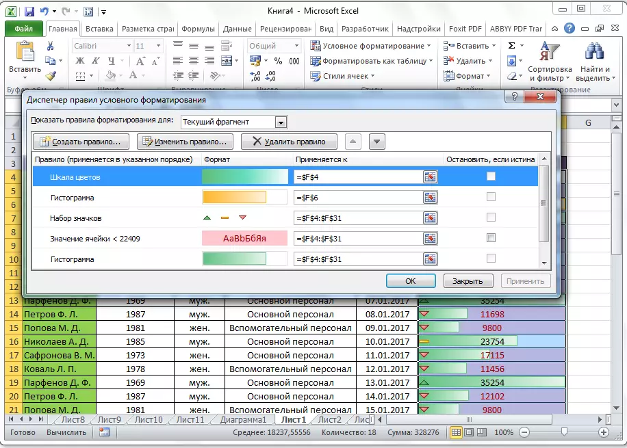
To change the rules in places, there are buttons in the form of arrows directed up and down. In order for the rule to be displayed on the screen, you need to highlight it, and press the button in the form of an arrow directionally down, until the rule does not take the latest line in the list.

There is another option. You need to install a tick in the column with the name "Stop, if the Truth" opposite the rules we need. Thus, turning over the rules from top to bottom, the program will stop on the rule, about which this mark costs, and will not fall below, which means that this rule will actually be performed.

In the same window, there are buttons for creating and changing the selected rule. After clicking on these buttons, the windows of the creation and change of the rules are launched, which we have already mentioned above.
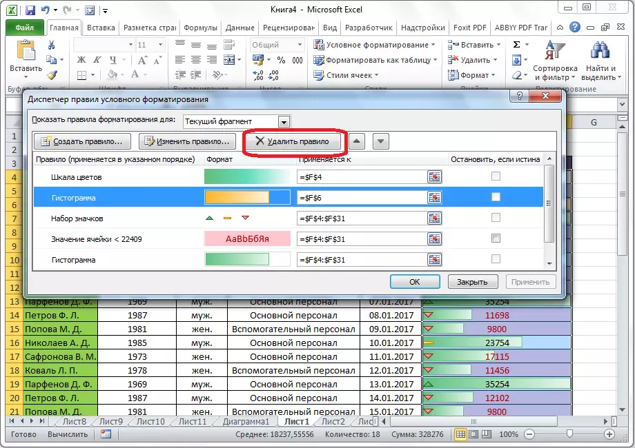
In order to delete the rule, you need to highlight it, and click on the "Delete Rule" button.
In addition, you can delete rules and through the main conditional formatting menu. To do this, click on "Delete Rules". Opens a submenu where you can select one of the options for deletion: Either delete the rules only on the dedicated range of cells, or delete absolutely all the rules that are available on the Excel open sheet.

As you can see, conditional formatting is a very powerful tool for visualizing data in the table. With it, you can configure the table in such a way that the general information on it will be assisted by the user at first sight. In addition, conditional formatting gives a great aesthetic appeal to the document.