How to make a calendar in Excel: 3 simple ways

When creating tables with a specific data type, sometimes you need to apply a calendar. In addition, some users simply want to create it, print and use for domestic purposes. The Microsoft Office program allows multiple ways to insert a calendar into a table or on a sheet. Let's find out how it can be done.

Creating various calendars

All calendars created in Excel can be divided into two large groups: covering a certain period of time (for example, year) and the eternal, which will be updated themselves at the current date. Accordingly, the approaches to their creation are somewhat different. In addition, you can use the ready template.

Method 1: Creating a calendar for a year

First of all, consider how to create a calendar for a certain year.

1. We develop a plan, as it will look, where it will be placed, which orientation to have (landscape or book), we determine where the days of the week will be written (side or top) and solve other organizational issues.
2. In order to make the calendar for one month allocate an area consisting of 6 cells in the height and 7 cells in width, if you decide to write the days of the week from above. If you write them to the left, then, accordingly, on the contrary. Being in the "Home" tab, click on the tape on the "Border" button, located in the Font Tool Block. In the list that appears, select the item "All Borders".



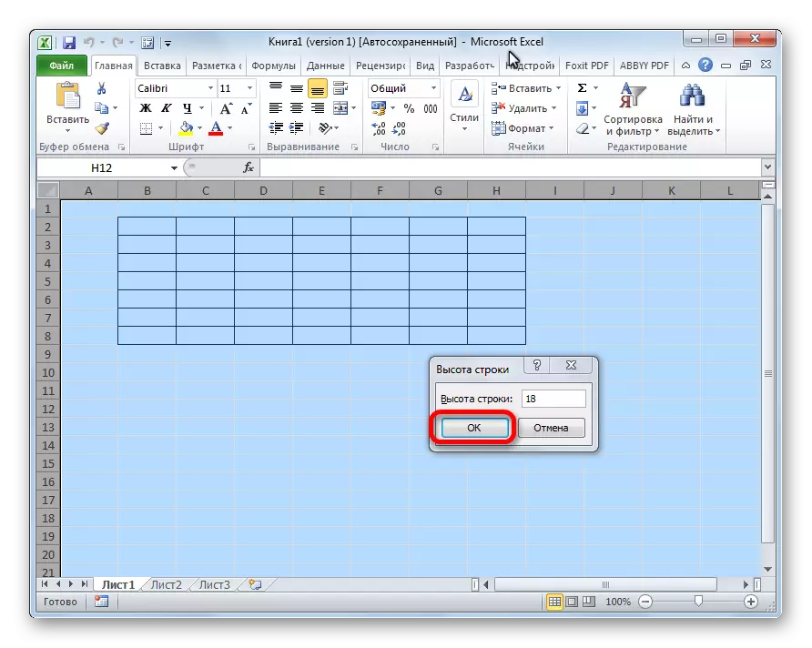
3. Align the width and height of the cells so that they take the square shape. In order to set the height of the row by clicking on the keyboard, the Ctrl + A keys. Thus, all the sheet stands out. Then call the context menu with the click of the left mouse button. Select the item "Line height".

   

   A window opens in which you want to set the required row height. Food you first make a similar operation and do not know what size to install, put 18. Then click on the "OK" button.

   

   Now you need to set the width. Click on the panel, on which the names of the columns are given to the letters of the Latin alphabet. In the menu that appears, select the "Column Width" item.

   

   In the window that opens, set the desired size. If you do not know what size to install, you can put a digit 3. Click on the "OK" button.

   

   After that, the cells on the sheet will acquire a square form.

4. Now we need to reserve a place for the name of the month. Select cells that are above the string of the first element for the calendar. In the "Home" tab in the "Alignment" tool block, press the "Combine and Place in the Center" button.



5. We prescribe the days of the week in the first row of the calendar element. This can be done using autofill. You can also format the cells of this small table at your discretion, so that it does not have to format each month separately. For example, you can pour a column designed for Sundays in red, and the text of the string in which the names of the week of the week are located, make a bold.



6. Copy the calendar elements for another two months. At the same time, we do not forget that the combined cell above the elements also entered the copying area. Insert them into one row so that between the elements there is a distance in one cell.



7. Now we highlight all these three items, and copy them down another three rows. Thus, it should be a total of 12 elements for each month. Distance between rows make two cells (if you use a book orientation) or one (when using landscape orientation).



8. Then in the combined cell we write the name of the month over the template of the first element of the calendar - "January". After that, we prescribe your name for each subsequent element.



9. At the final stage, we put the date in the cells. At the same time, it is possible to significantly reduce the time, using the autocomplete function, the study of which is devoted to a separate lesson.

After that, we can assume that the calendar is ready, although you can additionally format it at your discretion.

Lesson: How to make autocomplete in Excel

Method 2: Creating a calendar using formula

But, after all, the previous method of creation has one significant drawback: it will have to re-on every year. At the same time, there is a way to insert a calendar in Excel with the help of the formula. It will be updated every year. Let's see how it can be done.

1. Insert the function to the left top cell:

   = "Calendar on" & Year (today ()) & "Year"

   Thus, we create a calendar header with the current year.



2. Blackcraft patterns for the elements of the calendar monthly, as well as we did in the previous method with a passing change in the magnitude of the cells. You can immediately format these elements: fill, font, etc.



3. To the place where the names of the month "January" should be displayed, insert the following formula:

   = Date (year (today ()); 1; 1)

   

   But, as you can see, in the place where the name should be displayed simply the date was set. In order to bring the cell format to the desired form, click on it right-click. In the context menu, select the item "Format cells ...".

   

   In the opened cell format window, go to the "Number" tab (if the window opened in another tab). In the "Numeric formats" block allocate the "Date" item. In the "Type" block, select the MART value. Do not worry, this does not mean that the word "March" will be in the cell, since this is just an example. Click on the "OK" button.



4. As we see, the name in the header of the calendar element has changed to "January". In the header of the next item insert another formula:

   = Datime (B4; 1)

   In our case, B4 is the address of the cell with the name "January". But in each particular case, the coordinates may be different. For the next element, I will already refer not to "January", but to "February", etc. We format the cell in the same way as it was in the previous case. Now we have the names of months in all the elements of the calendar.



5. We should fill in the dates field. We allocate in the calendar element for January all cells intended for making dates. In the formula string, we drive the following expression:

   = Date (year (D4); month (D4); 1-1) - (time (date (year (D4); month (D4); 1-1)) - 1) + {0: 1: 2: 3 : 4: 5: 6} * 7 + {1; 2; 3; 4; 5; 6; 7}

   Click the combination of keys on the keyboard Ctrl + SHIFT + ENTER.



6. But, as we see, the fields were filled with incomprehensible numbers. In order for them to take the form we need. We format them under the date, as it has already done earlier. But now in the "Numeric formats" block, select "All Formats". In the "Type" block, the format will have to be administered manually. There we are simply the letter "D". Click on the "OK" button.



7. We drive out similar formulas into the calendar elements for other months. Only now, instead of the address of the D4 cell in the formula, it will be necessary to put the coordinates with the name of the cell name of the corresponding month. Then, we perform formatting in the same way that we are described above.



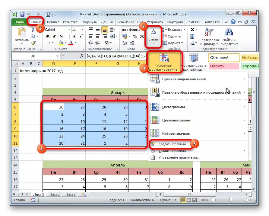
8. As you can see, the location of the dates in the calendar is still not correct. In one month should be from 28 to 31 days (depending on the month). We also have numbers from the previous and subsequent month in each element. They need to be removed. Apply conditional formatting for these purposes.

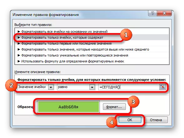
   We produce in the calendar block for January, the selection of cells in which the numbers are contained. Click on the "Conditional Formatting" icon posted on the tape in the "Home" tab in the "Styles" tool block. In the list that appears, select the value "Create Rule".

   

   A conventional formatting rule window opens. Select the type "Use the formula to determine the formatable cells". Insert the formula to the corresponding field:

   = And (month (D6) 1 + 3 * (private (string (D6) -5; 9)) + private (column (D6); 9))

   D6 is the first cell of the allocated array that contains dates. In each case, its address may differ. Then click on the "Format" button.

   

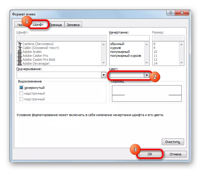
   In the window that opens, go to the "Font" tab. In the "Color" block, choose a white or color background if you have a calendar color background. Click on the "OK" button.

   

   Returning to the Create Rules window, click on the "OK" button.



9. Using a similar method, we carry out conditional formatting relative to other calendar elements. Only instead of the D6 cell in the formula will need to specify the address of the first cell of the range in the corresponding element.



10. As you can see, the numbers that are not included in the corresponding month merged with the background. But, in addition, weekends merged with him. This was done specifically, as the cells, where to contain the number of weekend days we will hinder in red. We allocate in the January block of the region, the numbers in which fall on Saturday and Resurrection. At the same time, we exclude those bands that were specifically hidden by formatting, as they relate to another month. On the tape in the "Home" tab in the "Font" tool block on the "Fill color" icon and choose a red color.

    

    Exactly the same operation is done with other elements of the calendar.



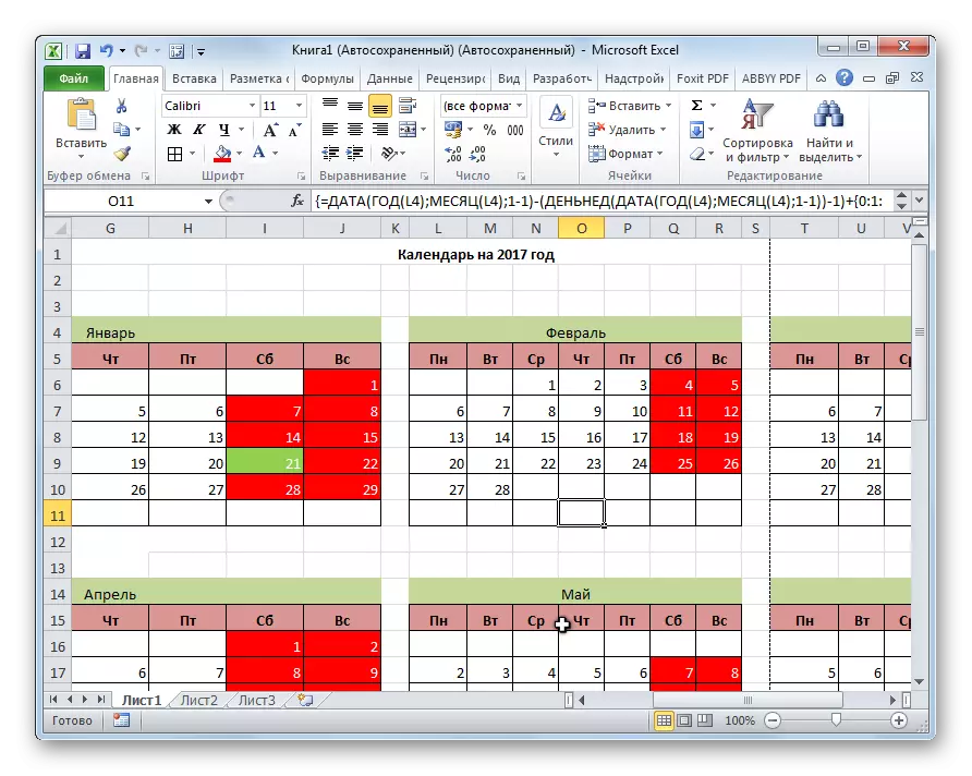
11. We will highlight the current date in the calendar. To do this, we will need to make the conditional formatting of all table items. This time I select the rule type "format only cells that contain". As a condition, we install the cell value to be equal to the current day. To do this, drive into the appropriate field formula (shown in the illustration below).

    = Today ()

    In the pouring format, select any color, different from the total background, for example green. Click on the "OK" button.

    

    After that, the cell corresponding to the current number will have a green color.

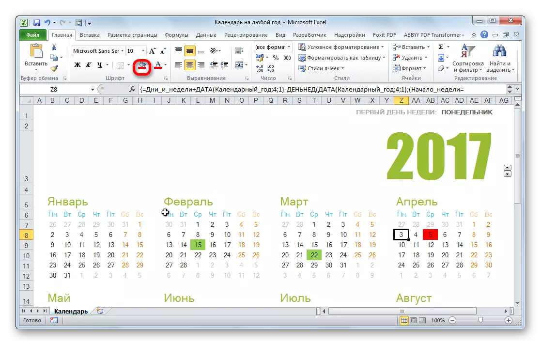
12. Set the name "Calendar for 2017" in the middle of the page. To do this, allocate the entire line, where this expression is contained. Click on the "Combine and Place the Center" button on the tape. This name for the total presentability can be additionally formatted in various ways.

In general, the work on the creation of the "eternal" calendar is completed, although you can take a long time to carry out various cosmetic work on it, editing the appearance of your taste. In addition, you can separately allocate, for example, holidays.

Lesson: Conditional formatting in Excel

Method 3: Usage Template

Those users who still have no extent own exceiver or simply do not want to spend time on creating a unique calendar, can take advantage of the finished pattern by uploaded from the Internet. There are quite a few such templates in the network, and not only the quantity, but also a variety. You can find them by simply by driven by the appropriate request to any search engine. For example, you can specify the following query: "Calendar Excel Template".

Note: In the latest versions of the Microsoft Office package, a huge selection of templates (including calendars) is integrated into software products. All of them are displayed directly when opening the program (not a specific document) and, for more user friendly, divided into thematic categories. It is here that you can choose a suitable template, and if it does not have any, it can always be downloaded from the official website of Office.com.

In fact, such a template is already a ready calendar in which you will only stay to drive holiday dates, birthdays or other important events. For example, such a calendar is a template that is presented in the image below. It is a fully finished table.

You can use the fill button in the "Home" tab, paint the different colors of the cells in which the dates are contained, depending on their importance. Actually, all the work with a similar calendar can be considered over and they can begin to use.

We figured out that the calendar in Excele can be made in two main ways. The first one implies the execution of almost all actions manually. In addition, the calendar made in this way will have to update every year. The second method is based on the application of formulas. It allows you to create a calendar that will be updated myself. But, for the use of this method in practice, you need to have greater luggage knowledge than when using the first option. Knowledge of the application of such a tool as conditional formatting will be especially important. If your knowledge is minimal in Excel, you can use the finished template downloaded from the Internet.