

When working with Excel tables, sometimes you need to hide certain areas of the sheet. Quite often, this is done if there are formulas in them. Let's find out how to hide the columns in this program.
Algorithms hide
There are several options to perform this procedure. Let's find out what their essence is.Method 1: Cell shift
The most intuitive option, with which you can achieve the desired result, is the cell shift. In order to produce this procedure, we bring the cursor to the horizontal coordinate panel in the place where the border is located. An arrow characteristic appears in both directions. We click on the left mouse button and drag the boundaries of one column to the borders of another, as far as it can be done.
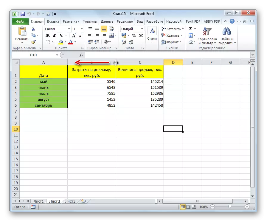
After that, one element will actually hidden after another.
Method 2: Using the context menu
It is more convenient for these goals to use the context menu. First, it is easier than moving the borders, secondly, thus, it is possible to achieve full hide cells, in contrast to the previous version.
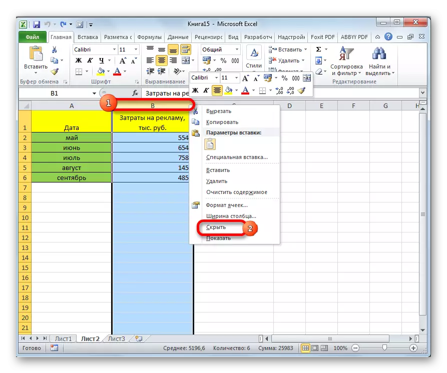
- With the right mouse button on the horizontal coordinate panel in the area of the Latin letter, which the column is denoted to be hidden.
- In the context menu that appears, click on the "Hide" button.
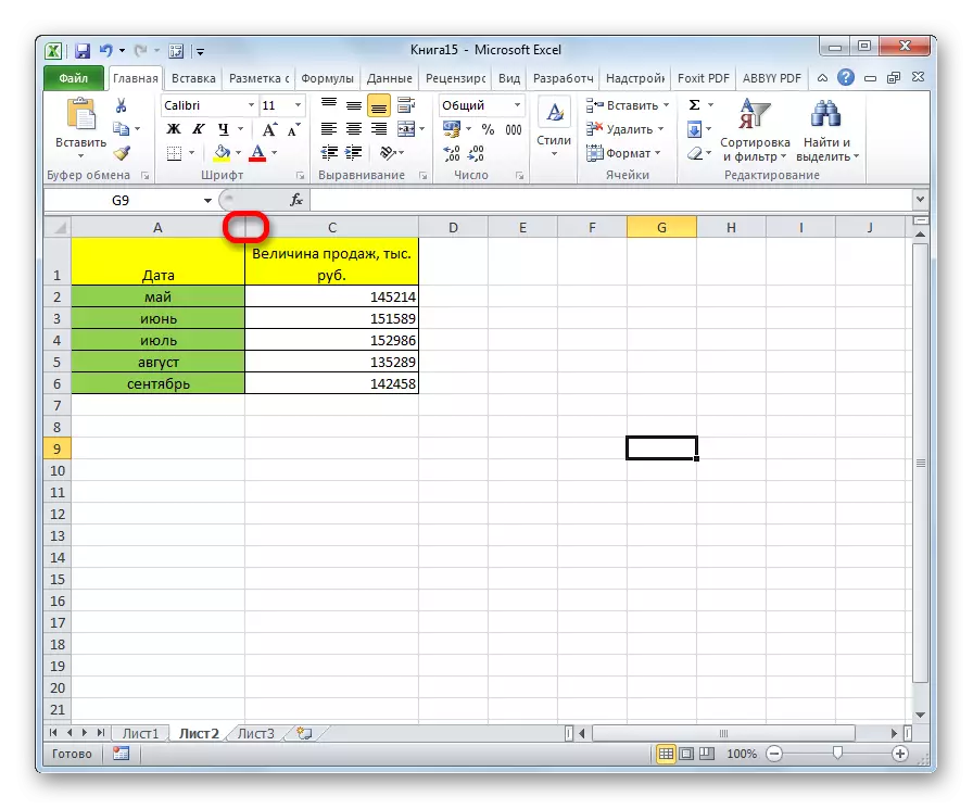
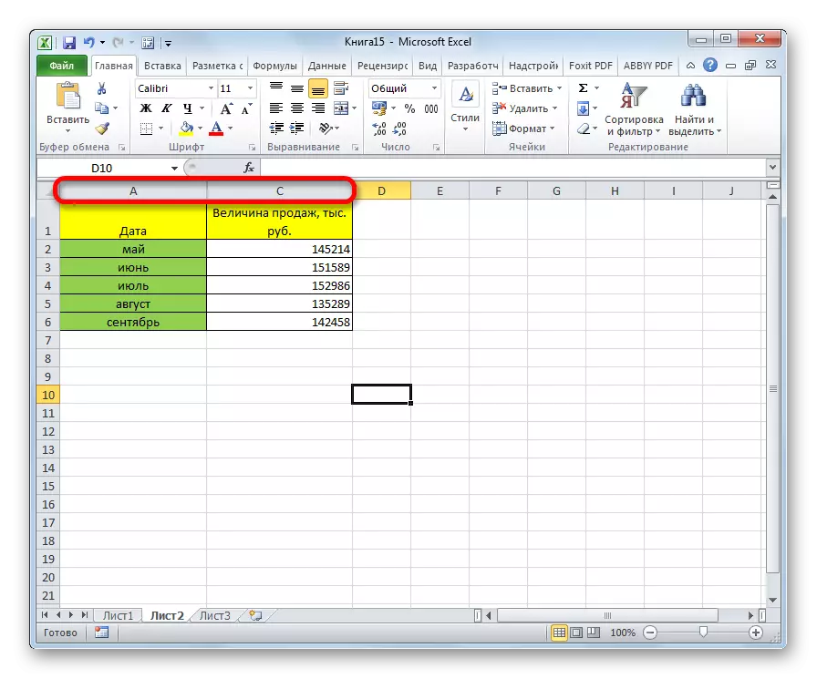
After that, the specified column will be completely hidden. In order to make sure that, take a look at how the columns are indicated. As you can see, in a consistent manner, there is not enough one letter.
The advantages of this method before the previous one lies in the fact that with it you can hide several sequentially located columns simultaneously. To do this, you need to highlight them, and in the resulting context menu, click on the "Hide" item. If you want to produce this procedure with elements that are not located next to each other, but scattered on the sheet, then the selection must be carried out with the CTRL button on the keyboard.

Method 3: Using tape tools
In addition, you can execute this procedure using one of the tape buttons in the "Cell tools" block.
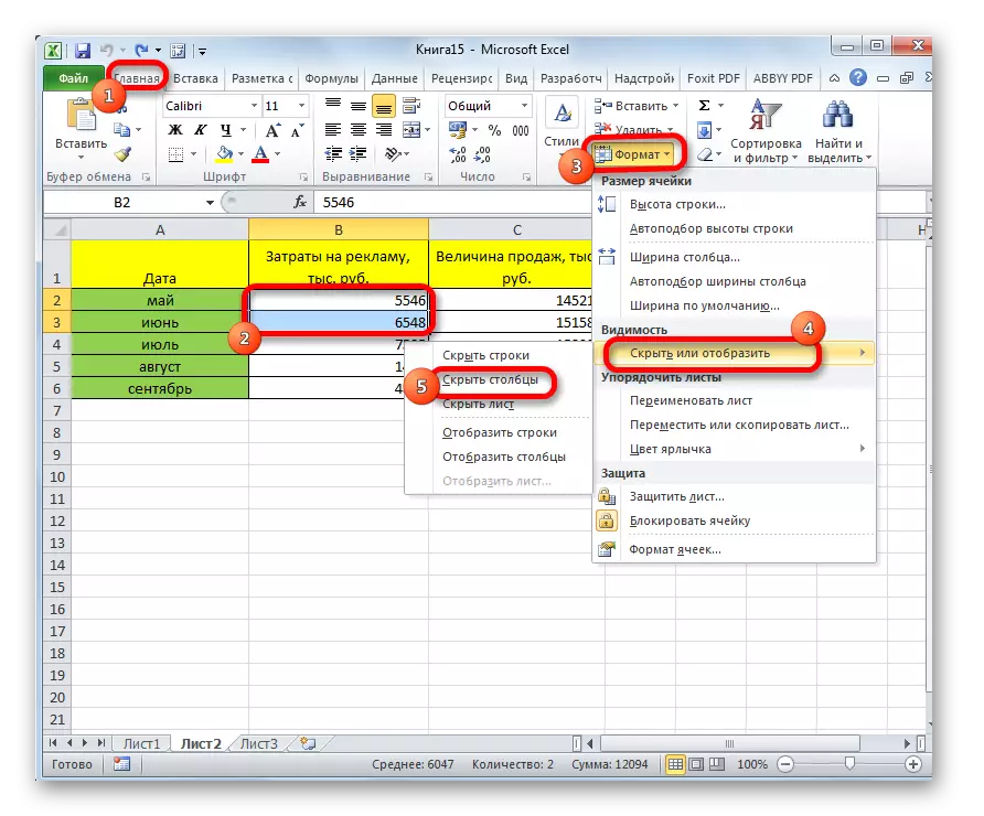
- Select cells located in columns to be hidden. Being in the "Home" tab, click on the "Format" button, which is located on the tape in the block of the "Cell tools". In the menu that appears in the "Visibility" settings group, click on the "Hide or Display" item. Another list is activated in which you want to select "Hide Columns".
- After these actions, the columns will be hidden.
As in the previous case, therefore, you can hide several elements at once, allocating them, as described above.
Lesson: How to display hidden columns in Excel
As you can see, there are several ways to hide the columns in the Excel program. The most intuitive method is the shift of cells. But it is also recommended to use one of the two following options (context menu or tape button), as they guarantee that cells will be completely hidden. In addition, the elements thus hidden then will be easier to display back when necessary.