

When working with tables, which includes a large number of rows or columns, the question of data structuring becomes relevant. In Excel, this can be achieved by using the grouping of the corresponding elements. This tool allows not only conveniently structuring data, but also to temporarily hide unnecessary elements, which allows you to concentrate your attention on other parts of the table. Let's find out how to produce a group in Excele.
Setting up grouping
Before proceeding to grouping rows or columns, you need to configure this tool so that the end result is close to the user expectations.
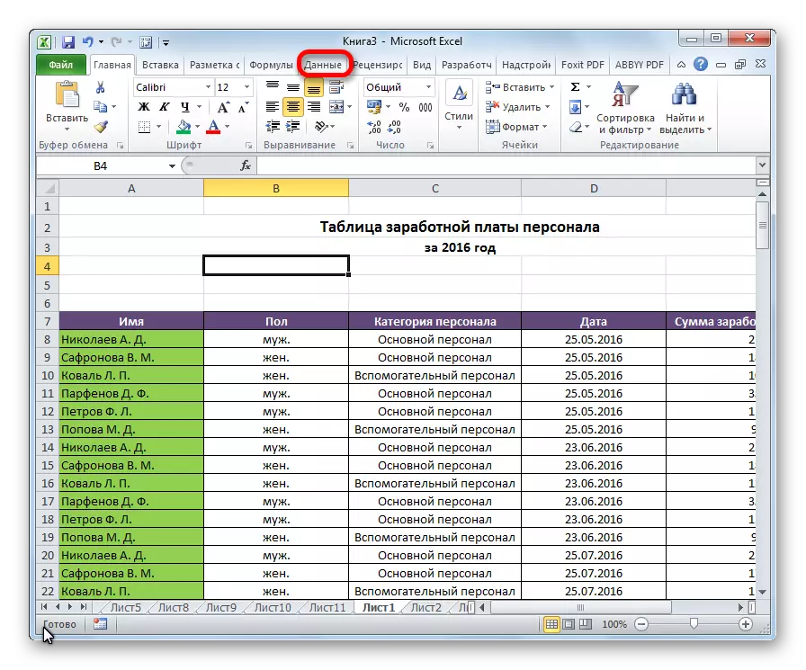
- Go to the "Data" tab.
- In the lower left corner of the "Structure" tool block on the ribbon there is a small inclined arrow. Click on it.
- A group setup window opens. As we see by default it is established that the results and names on the columns are located to the right of them, and on the rows - below. It does not suit many users, as it is more convenient when the name is placed on top. To do this, you need to remove a tick from the corresponding item. In general, each user can configure these parameters for itself. In addition, you can immediately include automatic styles by installing a tick near this name. After the settings are exhibited, click on the "OK" button.


On this setting the grouping parameters in Excel is completed.
Grouping on strings
Perform a grouping of data on lines.
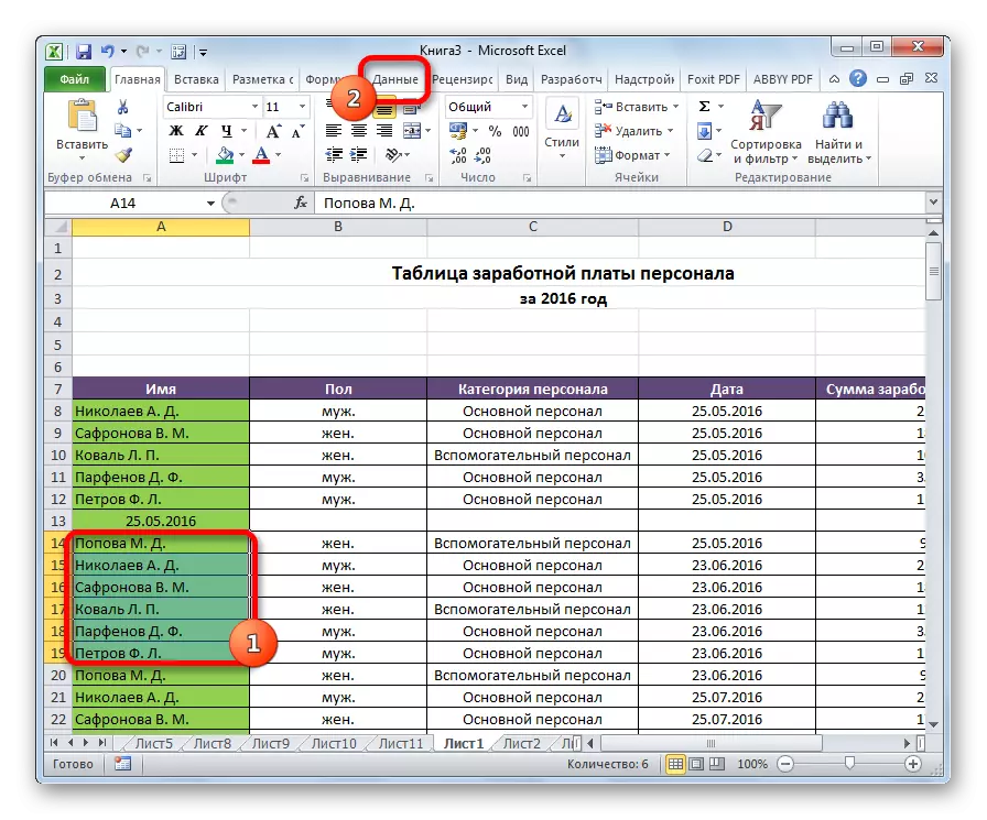
- Add a line over a group of columns or under it, depending on how we plan to display the name and results. In the new cell we introduce an arbitrary name of the group, suitable for it by context.
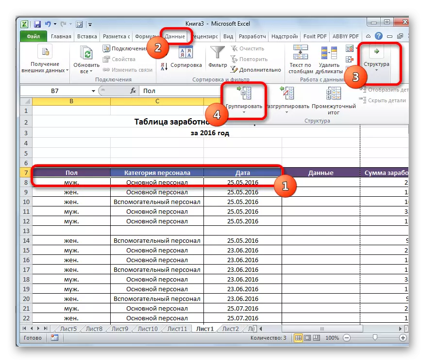
- We highlight the lines that need to be grouped, in addition to the final string. Go to the "Data" tab.
- On the tape in the "Structure" tool block by clicking on the "Grind" button.
- A small window opens in which you need to answer that we want to group - strings or columns. We put the switch to the "string" position and click on the "OK" button.


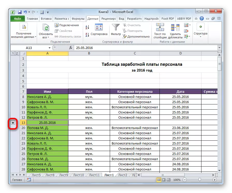
This creation has been completed on this. In order to roll it enough to click on the "minus" sign.

To re-deploy a group, you need to click on the plus sign.
Grouping on columns
Similarly, the grouping on columns is carried out.
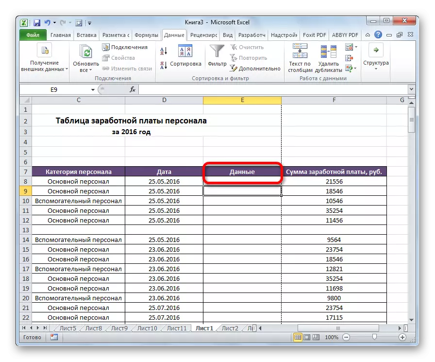
- On the right or left of the groupable data, add a new column and indicate in it the corresponding name of the group.
- Select cells in columns that are going to group, except the column with the name. Click on the "Grind" button.
- In the window that opens this time, we put the switch to the "columns" position. Click on the "OK" button.

The group is ready. Similarly, as when grouping columns, it can be folded and deployed by clicking on the "minus" and "plus" signs, respectively.
Creating nested groups
In Excel, you can create not only first-order groups, but also invested. For this, it is necessary in the deployment of the parent group to highlight certain cells in it, which you are going to groupe separately. Then it should be done one of those procedures that were described above, depending on whether you work with columns or with rows.
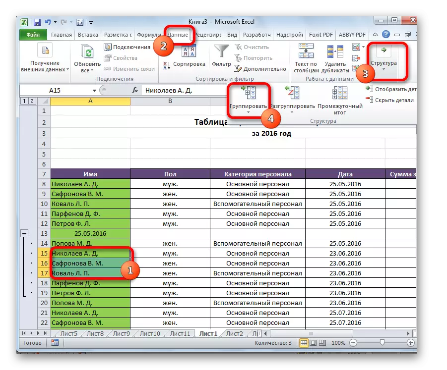
After that, the nested group will be ready. You can create an unlimited number of similar attachments. Navigation between them is easy to spend, moving through the numbers located on the left or on top of the sheet, depending on which the string or columns are grouped.

Lust
If you want to reformat or simply delete a group, it will need to be ungraved.
- Select cells of columns or lines that are subject to ungrouping. Click on the "Ungroup" button, located on the tape in the "Structure" settings block.
- In the appeared window, we choose what exactly we need to disconnect: rows or columns. After that, we click on the "OK" button.


Now the dedicated groups will be disbanded, and the sheet structure will take its original appearance.
As you can see, create a group of columns or rows is quite simple. At the same time, after this procedure, the user can make it easier to work with a table, especially if it is very big. In this case, the creation of nested groups can also help. To carry out ungraveing as simple as data grouped.