How to calculate the variation coefficient in Excel

One of the main statistical indicators of the sequence of numbers is the variation coefficient. To find it is quite complex calculations. Microsoft Excel tools allow you to significantly alleviate them for the user.

Calculation of the coefficient of variation

This indicator is the ratio of a standard deviation to the middle arithmetic. The result obtained is expressed as a percentage.

Excel does not separately exist functions for calculating this indicator, but there are formulas for calculating the standard deviation and an average arithmetic series of numbers, namely they are used to find the coefficient of variation.

Step 1: Calculation of standard deviation

Standard deviation, or, as it is called differently, the standard deviation is a square root from the dispersion. To calculate the standard deviation, the Standotclone function is used. Starting with the Excel 2010 version, it is divided, depending on whether the general set is calculated or by sample, two separate options: Standotclone.g and Standotclona.B.

The syntax of these functions looks accordingly:

= Standotclone (number1; number2; ...)

= Standotclonal.g (number1; number2; ...)

= Standotclonal.V (number1; number2; ...)

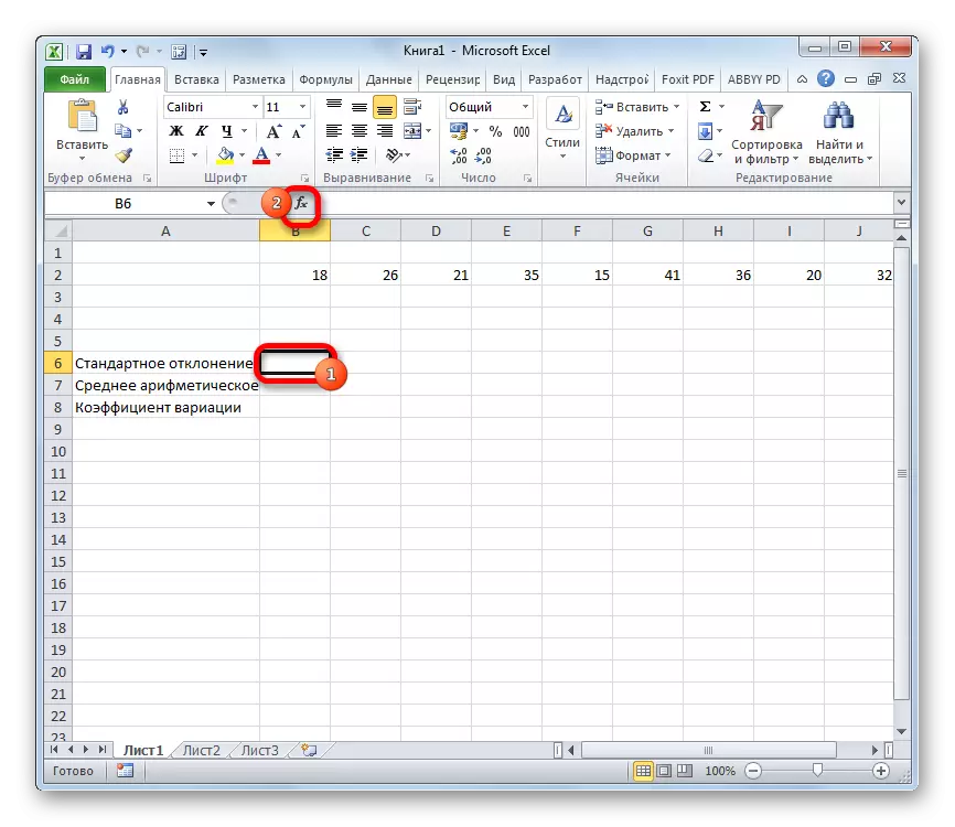
1. In order to calculate the standard deviation, select any free cell on the sheet, which is convenient for you in order to display the results of calculations. Click on the button "Paste a function". It has an appearance of the pictogram and is located on the left of the formula string.



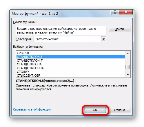
2. The activation of the wizard of functions is performed, which is started as a separate window with a list of arguments. Go to the category "Statistical" or "Full Alphabetical List". We choose the name "Standotclonal.g" or "Standotclona.V.", depending on whether the general combination or by the sample should be calculated. Click on the "OK" button.



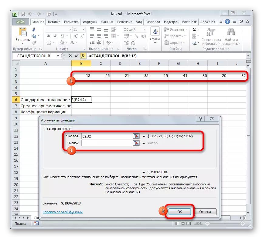
3. The arguments window opens. It can have from 1 to 255 fields, in which there are both specific numbers and references to cells or ranges. We put the cursor in the "Number1" field. Mouse allocate the range of values ​​to be processed on the sheet. If there are several such areas and they are not adjacent to each other, the coordinates of the following indicate the "Number2" field, etc. When all the necessary data is entered, click on the "OK" button



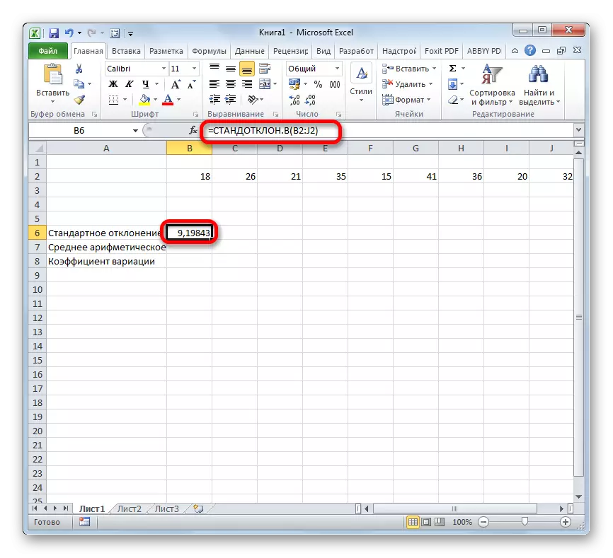
4. In the pre-selected cell, the total calculation of the selected type of standard deviation is displayed.

Lesson: Middle Quadratic Deviation Formula in Excel

Step 2: Calculation of the average arithmetic

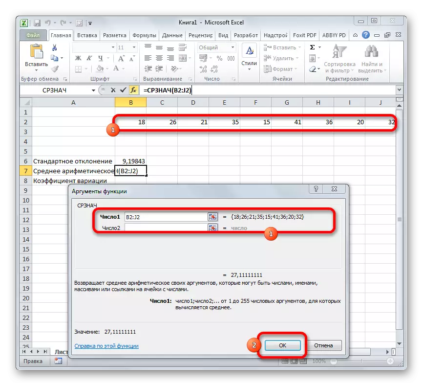
The arithmetic average is the ratio of the total amount of all values ​​of the numerical series to their quantity. To calculate this indicator, there is also a separate function - CPNPH. Calculate its value on a specific example.

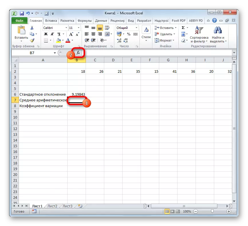
1. Select the cell on the sheet to output the result. We click on the "Insert function" button already familiar to us.



2. In the statistical category of the wizard of functions, we are looking for the name "SRNVOV". After it is selected, press the "OK" button.



3. The Argument window is launched. The arguments are completely identical to the fact that the operators of the Standotclone group. That is, in their quality can act as separate numeric values ​​and links. Install the cursor in the "Number1" field. Also, as in the previous case, we allocate the set of cells on the sheet. After their coordinates were listed in the window of the argument window, click on the "OK" button.



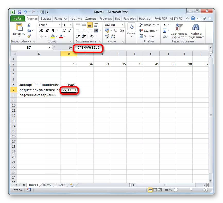
4. The result of calculating the average arithmetic is derived in the cell that was highlighted before opening the functions wizard.

Lesson: How to calculate the average value in Excel

Step 3: Finding the coefficient of variation

Now we have all the necessary data in order to directly calculate the variation coefficient itself.

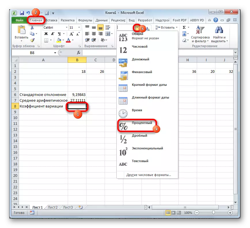
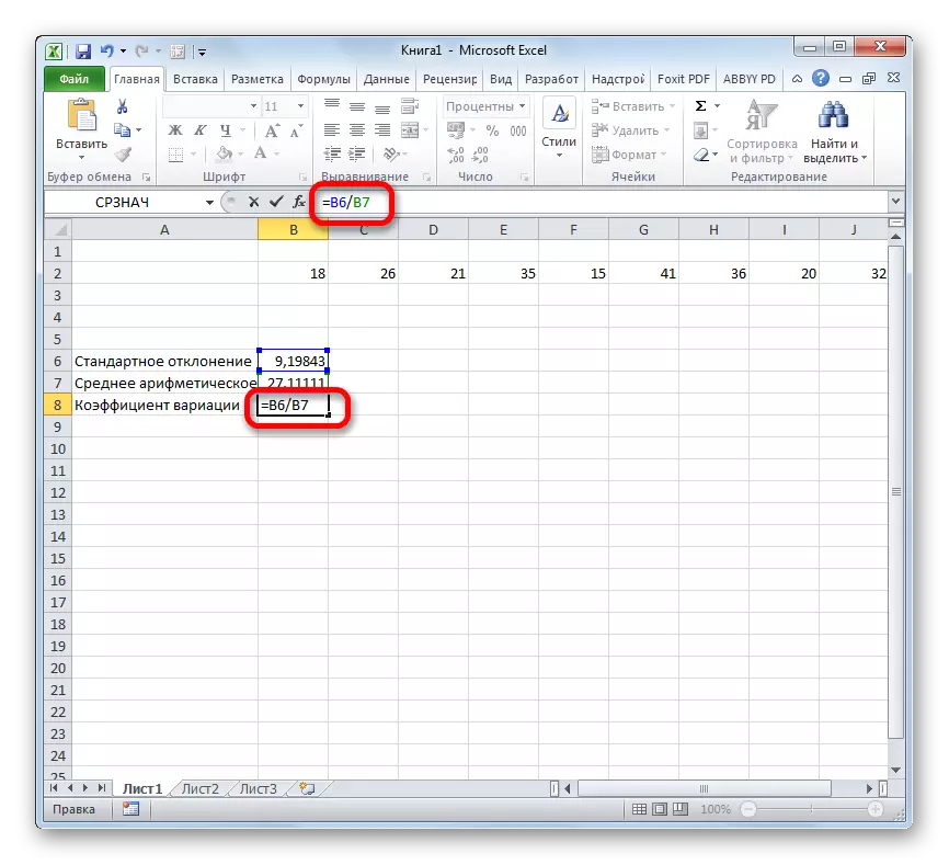
1. Select the cell into which the result will be displayed. First of all, it is necessary to consider that the variation coefficient is a percentage. In this regard, the cell format should be changed to the appropriate. This can be done after its selection, while in the "Home" tab. Click on the field of the format on the ribbon in the "Number" toolbar. From the discussed list of options, choose the "percentage". After these actions, the format at the element will be appropriate.



2. Returning back to the cell to display the result. Activate it with a double-click of the left mouse button. We put in it the sign "=". Select the element in which the outcome is the result of the calculation of the standard deviation. Click on the "split" button (/) on the keyboard. Next, we allocate the cell in which the arithmetic arithmetic set numerical series is located. In order to make the calculation and output, click on the ENTER button on the keyboard.



3. As you can see, the calculation result is displayed.

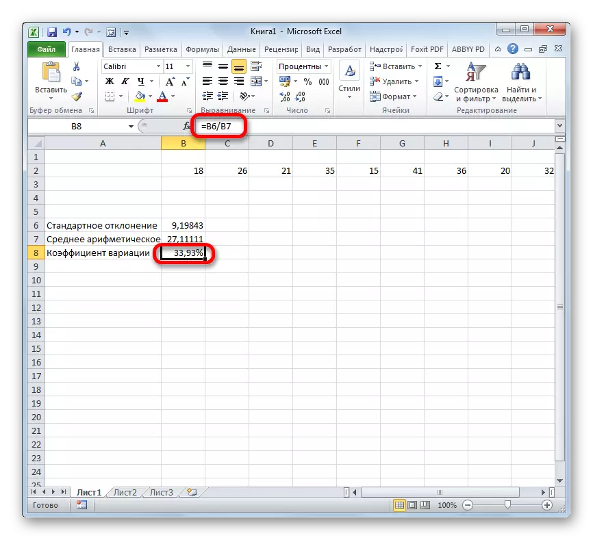
Thus, we have calculated the coefficient of variation, referring to the cells in which the standard deviation and arithmetic averages have already been calculated. But you can proceed and somewhat differently, without calculating these values.

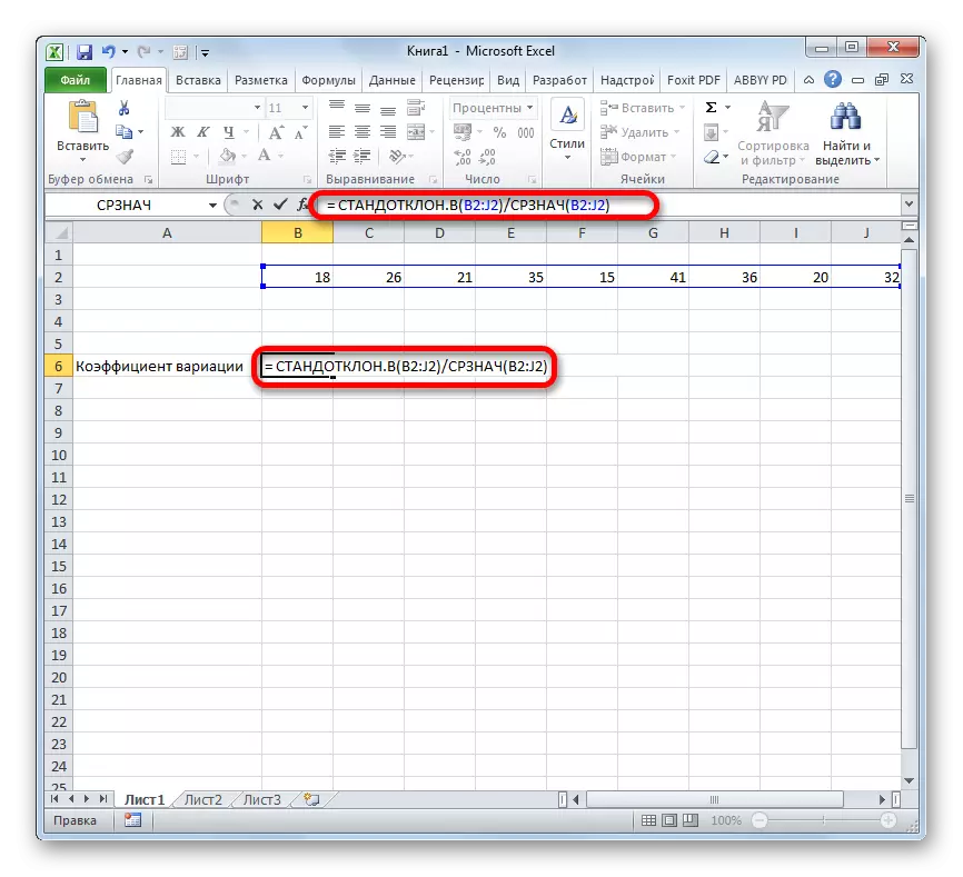
1. Select the cell previously formatted under the percentage format in which the result will be derived. We prescribe a type formula in it:

   = Standotclonal.V (range_name) / SR will (range_name)

   Instead of the name of the "range range" insert the real coordinates of the region, in which the numerical series has been placed. This can be done by simple allocation of this range. Instead of the Standotclonal Operator. In, if the user considers it necessary, the standard StandClon function can be used.



2. After that, to calculate the value and show the result on the monitor screen, click on the ENTER button.

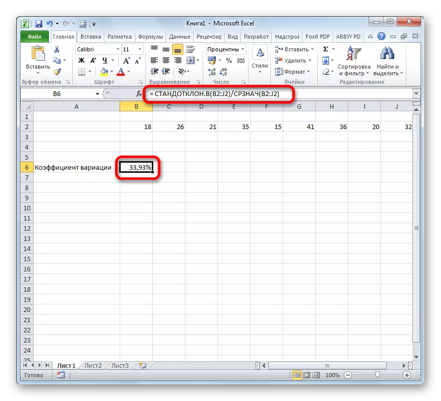
There is a conditional distinction. It is believed that if the indicator of the coefficient of variation is less than 33%, then the set of numbers is homogeneous. In the opposite case, it is customary to characterize as heterogeneous.

As you can see, the Excel program allows you to significantly simplify the calculation of such a complex statistical calculation as the search for the variation coefficient. Unfortunately, the appendix does not yet exist a function that would calculate this indicator in one action, but with the help of standard-clone operators, this task is very simplified. Thus, in Excel, even a person who does not have a high level of knowledge associated with statistical patterns can be performed.