

When working with data, it often arises the need to find out what place it takes in the aggregate list of one or another indicator. In statistics, this is called ranking. Excel has tools that allow users to quickly and easily produce this procedure. Let's find out how to use them.
Ranking functions
For ranking in Excel, special functions are provided. In the old versions of the application there was one operator designed to solve this task - rank. For compatibility purposes, it is left in a separate category of formulas and in modern versions of the program, but it is still desirable to work with newer analogues if there is such an opportunity. These include statistical operators Rang.rv and Rang.Sr. We will talk about differences and algorithm of work with them.Method 1: Rang.RV function
Operator Rang.RV produces data processing and displays the sequence number of the specified argument to the specified cell from the cumulative list. If multiple values have the same level, the operator displays the highest of the list of values. If, for example, two values will have the same value, then both will be assigned the second number, and the value of the value will have the fourth. By the way, the operator rank in older versions of Excel is completely similar, so that these functions can be considered identical.
The syntax of this operator is written as follows:
= Rank.RV (number; reference; [order])
The arguments "Number" and "Reference" are mandatory, and "order" is optional. As an argument "Number" you need to enter a link to the cell where the value contains the sequence number of which you need to know. The "Reference" argument contains the address of the entire range that is ranked. The "order" argument may have two meanings - "0" and "1". In the first case, the countdown of the order is descending, and in the second - by increasing. If this argument is not specified, it is automatically considered to be zero.
This formula can be written manually, in the cell where you want to show the result of processing, but for many users it is convenient to set the functions wizard in the wizard window.
- We allocate the cell on the sheet to which the data processing result will be displayed. Click on the button "Paste a function". It is localized to the left of the formula string.
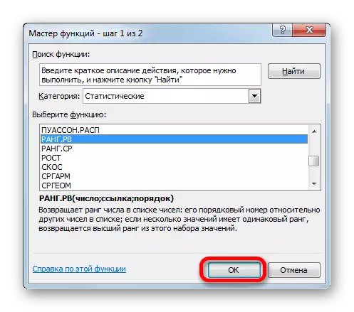
- These actions lead to the fact that the functions wizard window starts. It contains all (for rare exceptions) operators that can be used to compile formulas in Excel. In the category "Statistical" or "Full Alphabetical List" we find the name "Rang.RV", we allocate it and click on the "OK" button.
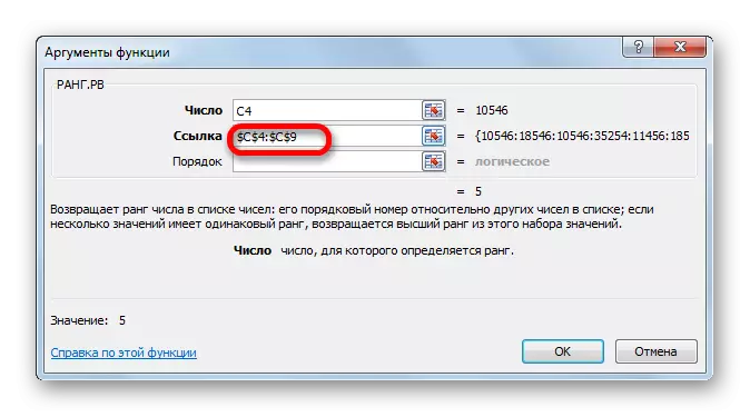
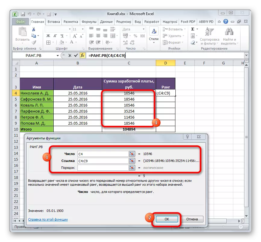
- After the above action, the function arguments will be activated. In the "Number" field, enter the address of that cell, the data in which you want to rank. This can be done manually, but it is more convenient to perform in the way that it will be discussed below. We establish the cursor in the "number" field, and then simply select the desired cell on the sheet.
After that, its address will be listed in the field. In the same way, we enter the data and in the link "Link", only in this case allocate the entire range, within which ranking occurs.
If you want the ranking to come from less to more, then in the "order" field should be set "1". If it is necessary that the order is distributed from greater to a smaller (and in the overwhelming number of cases it is necessary that it is necessary), then this field is left blank.
After all the above data is made, press the "OK" button.
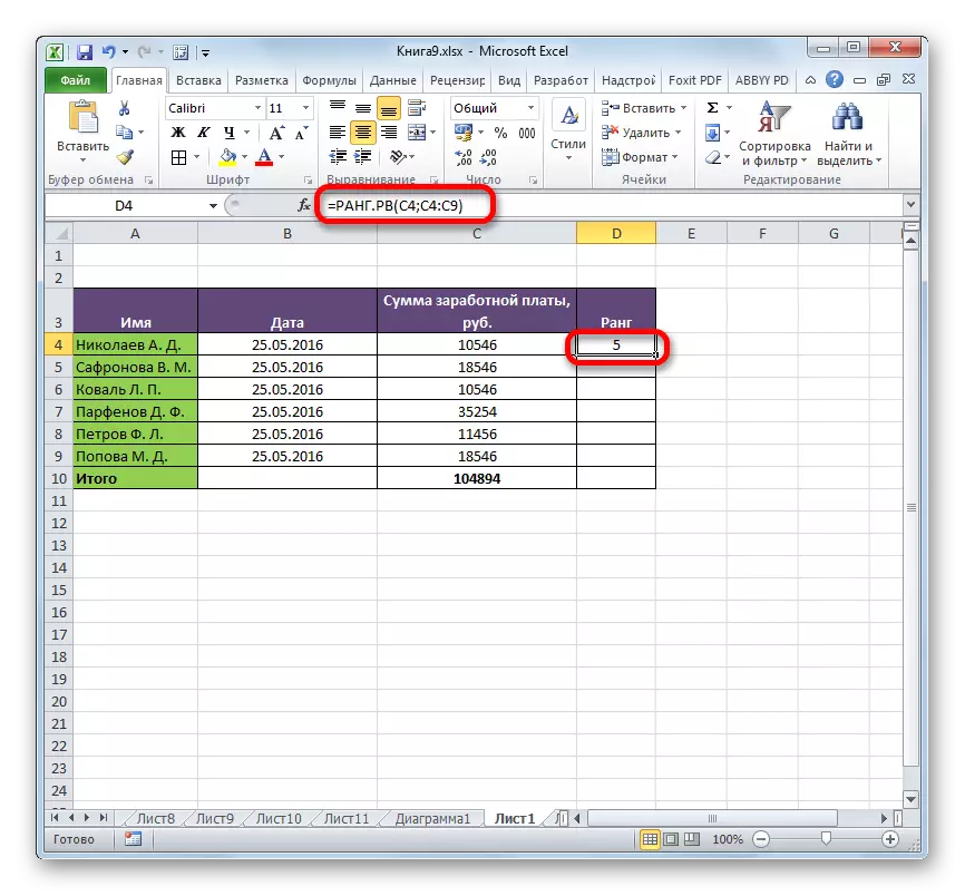
- After performing these actions in a pre-specified cell, the sequence number will be displayed, which has the value of your choice among the whole list of data.
If you wish to run the entire specified area, you do not need to enter a separate formula for each indicator. First of all, we make the address in the "Link" field. Before each coordinate value, add a dollar sign ($). At the same time, to change the values in the "Number" field to absolutely, in no case should not, otherwise the formula will be calculated incorrectly.
After that, you need to install the cursor in the lower right corner of the cell, and wait for the appearance of the filling marker in the form of a small cross. Then clamp the left mouse button and stretch the marker parallel to the calculated area.
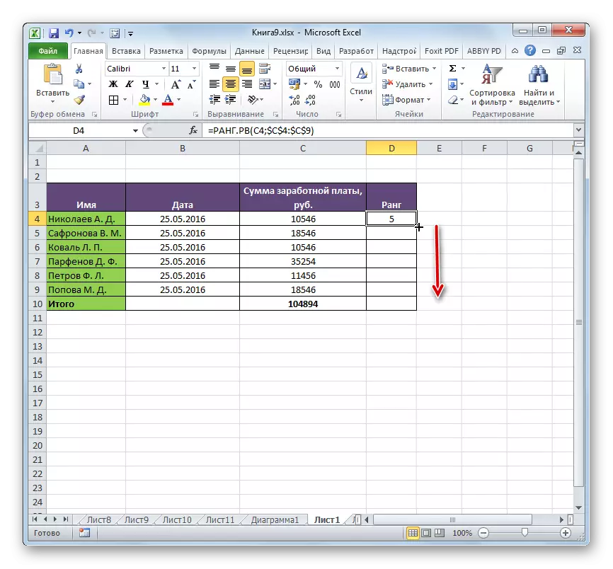
As we see, thus, the formula will be copied, and the ranking will be produced on the entire data range.

Lesson: Wizard Functions in Excel
Lesson: Absolute and relative links to Excel
Method 2: Function Rank.Sr
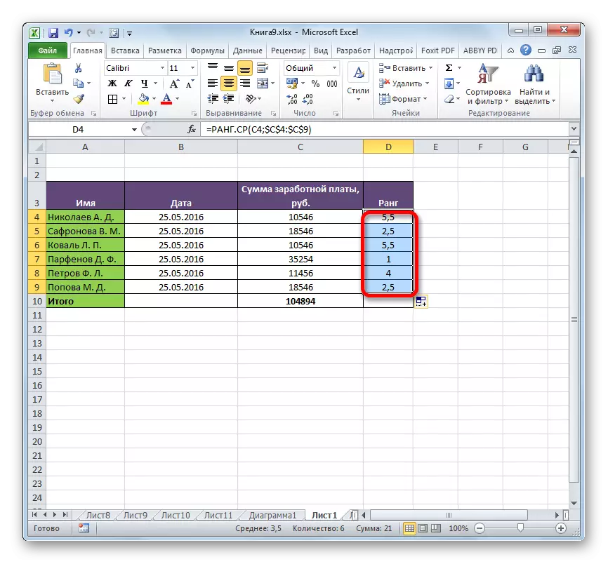
A second function that produces an operation of ranking in Excele is Rank.Sr. In contrast to the functions of rank and rank.RV, with the matches of the values of several elements, this operator issues an average level. That is, if two values have an equal value and follow after the value at number 1, then both of them will be assigned number 2.5.
Syntax Rank. SR is very similar to the diagram of the previous operator. He looks like this:
= Rank.Sr (number; reference; [Order])
The formula can be entered manually or through the functions master. In the last version we will stop more and dwell.
- We produce the selection of the cell on the sheet to output the result. In the same way, as in the previous time, go to the functions wizard through the "Insert function" button.
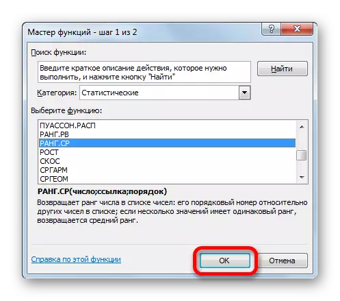
- After opening the window wizard window, we allocate the name of the "statistical" category "Statistical" name, and press the "OK" button.
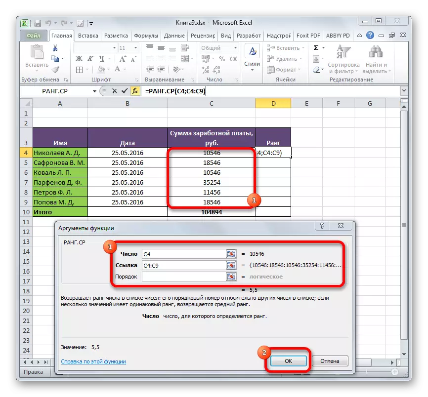
- The argument window is activated. The arguments of this operator are exactly the same as the function Rang.RV:
- Number (cell address containing an element whose level should be determined);
- Reference (Range coordinates, ranking inside which is performed);
- Order (optional argument).
Making data in the field occurs in exactly the same way as in the previous operator. After all the settings are made, click on the "OK" button.
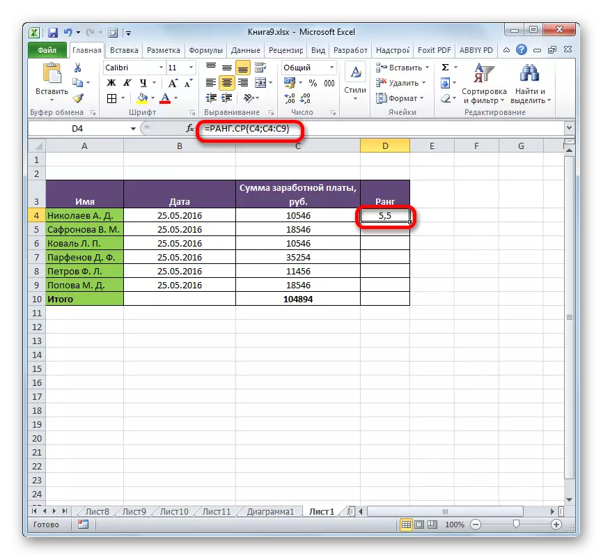
- As we can see, after completed actions, the calculation result was displayed in the cell marked in the first paragraph of this instruction. The result itself is a place that occupies a specific value among other values of the range. In contrast to the result, Rang.RV, the result of the operator Rank. CER may have a fractional value.
- As with the previous formula, by changing links from relative on the absolute and marker, the entire range of data can be run by auto-complete. The algorithm of action is exactly the same.
Lesson: Other statistical functions in Microsoft Excel
Lesson: How to make auto-filling in Excel
As you can see, there are two functions in Excel to determine the ranking of a specific value in the data range: Rang.RV and Rank.S. For older versions of the program, a rank operator is used, which is essentially a complete analogue of the Rang.RV function The main difference between the formula Rang.RV and Rank.Sras is that the first of them indicates the highest level with the coincidence of values, and the second displays the average in the form of a decimal fraction. This is the only difference between these operators, but it must be taken into account when choosing exactly which function the user is better to use it.