How to hide lines and cells in Excel

When working in Excel's program, it is quite often possible to find a situation where a significant part of the leaf array is used simply to calculate and does not bear the information load for the user. Such data only occupy a place and distract attention. In addition, if the user will accidentally break their structure, it can violate the entire calculation cycle in the document. Therefore, such rows or individual cells are better to hide. In addition, you can hide those data that is simply temporarily needed so that they do not interfere. Let's find out what methods it can be done.

Hiding procedure

Hide cells in Excele can be several completely different ways. Let us dwell on each of them so that the user himself can understand, in what situation it will be more convenient to use a specific option.

Method 1: Grouping

One of the most popular ways to hide the elements is their grouping.

1. We highlight the sheet lines that need to be grouped, and then hide. It is not necessary to allocate the entire string, and it can be noted only by one cell in the groupable lines. Next, go to the tab "Data". In the "Structure" block, which is located on the tape ribbon, press the "Grind" button.



2. A small window opens, which offers to choose what exactly needs to be grouped: rows or columns. Since we need to group rows, we do not produce any changes to the settings, because the default switch is set to the position that we need. Click on the "OK" button.



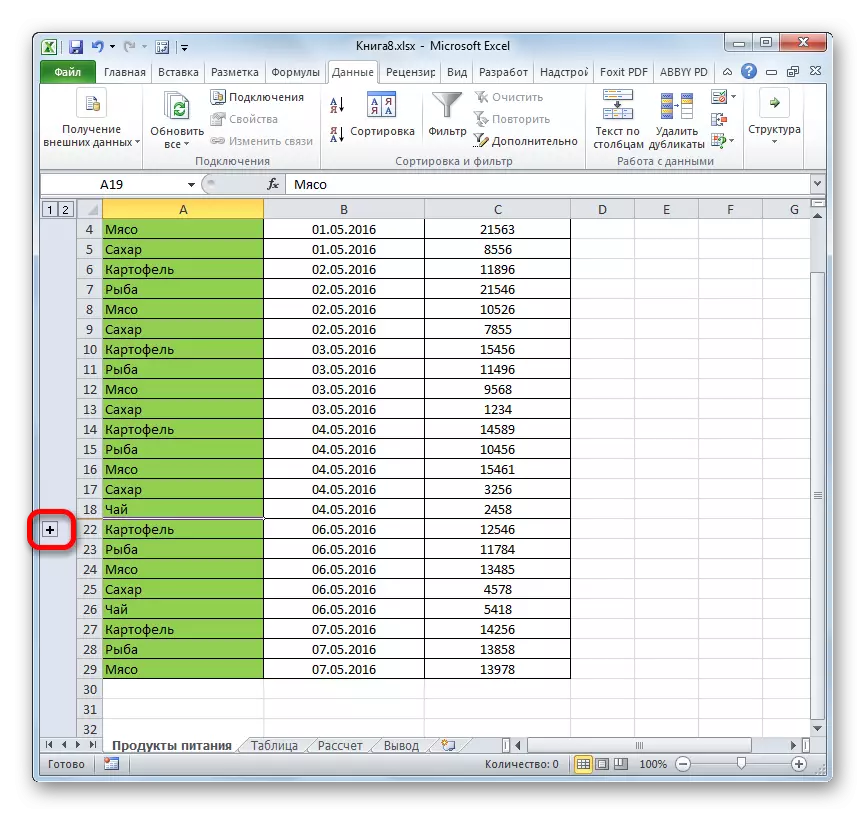
3. After that, a group is formed. To hide the data that is located in it is enough to click on the icon in the form of a "minus" sign. It is placed on the left of the vertical coordinate panel.



4. As you can see, the rows are hidden. To show them again, you need to click on the "plus" sign.

Lesson: How to make a grouping in Excel

Method 2: Thinking cells

The most intuitive way to hide the contents of the cells, probably, is to drag the boundaries of rows.

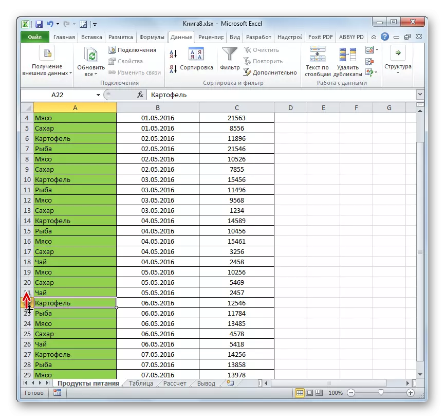
1. We establish the cursor on the vertical coordinate panel, where the rows numbers are marked, on the lower limit of that line, the contents of which we want to hide. In this case, the cursor must convert to the icon in the form of a cross with a double pointer, which is directed up and down. Then pin the left mouse button and pull the pointer up until the bottom and upper boundaries of the line do not close.



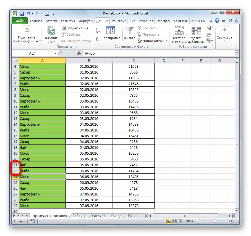
2. The string will be hidden.

Method 3: Group Hide Celling Treatment

If you need this method to hide several elements at once, then first should be allocated.

1. Close the left mouse button and highlight the coordinate on the vertical coordinate panel that we wish to hide.

   

   If the range is large, then select the items as follows: click the left button by the number of the first lines of the array on the coordinate panel, then climb the Shift button and click the last target number.

   

   You can even highlight several separate lines. To do this, for each of them, you need to click on the left mouse button with the ctrl pinch.



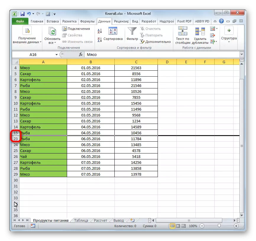
2. We become a cursor to the lower border of any of these rows and stretch it up until the boundaries are closed.



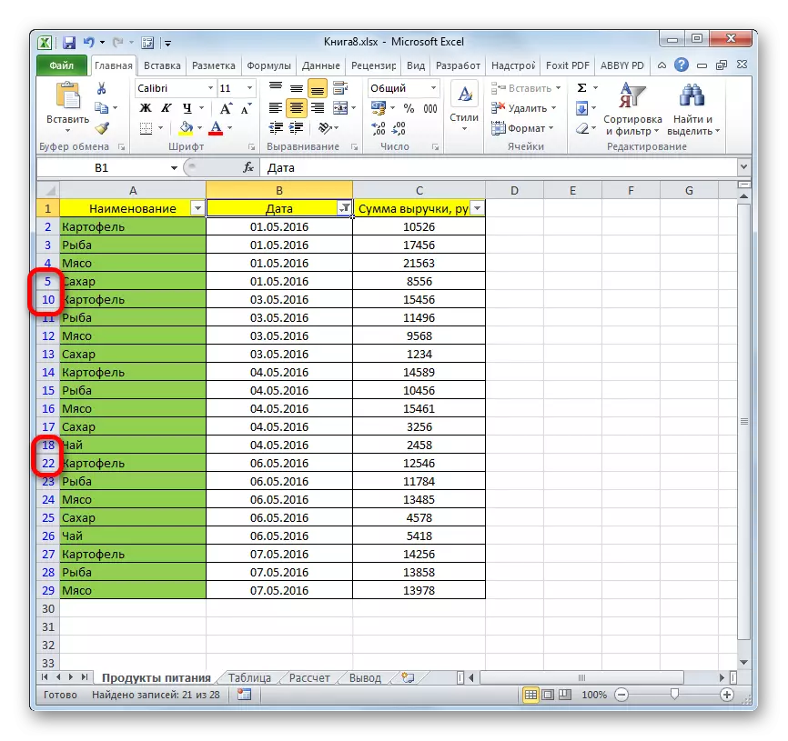
3. In this case, not only the string will be hidden, over which you work, but also all lines of the allocated range.

Method 4: Context Menu

The two previous methods, of course, are most intuitive and easy to use, but they still cannot provide full hide cells. There is always a small space, clinging for which you can turn the cell back. Fully hide the string is possible using the context menu.

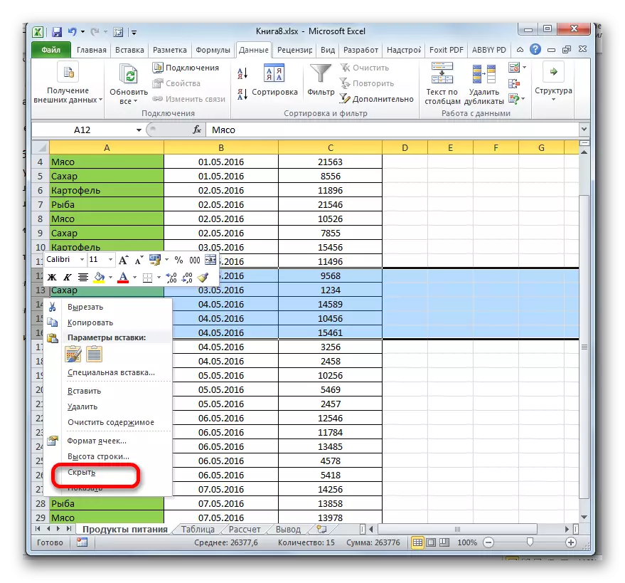
1. We highlight a line with one of the three ways that we are described above:
   • exclusively with the mouse;
   • using the SHIFT key;
   • Using the Ctrl key.



2. Click on the vertical scale of coordinates with the right mouse button. The context menu appears. We celebrate the item "Hide".



3. Selected lines due to the above actions will be hidden.

Method 5: Tool Tape

You can also hide the strings by using the button on the toolbar.

1. Select cells that are in the lines to be hidden. In contrast to the previous method, it is not necessary to allocate the entire line. Go to the "Home" tab. Click on the button on the Format Tool Ribbon, which is located in the "Cell" block. In the launched list, we bring the cursor to the only point of the group "Visibility" - "Hide or Display". In the additional menu, select the item that is needed to perform the target - "Hide lines".



2. After that, all the lines that contained the cell allocated in the first paragraph will be hidden.

Method 6: Filtering

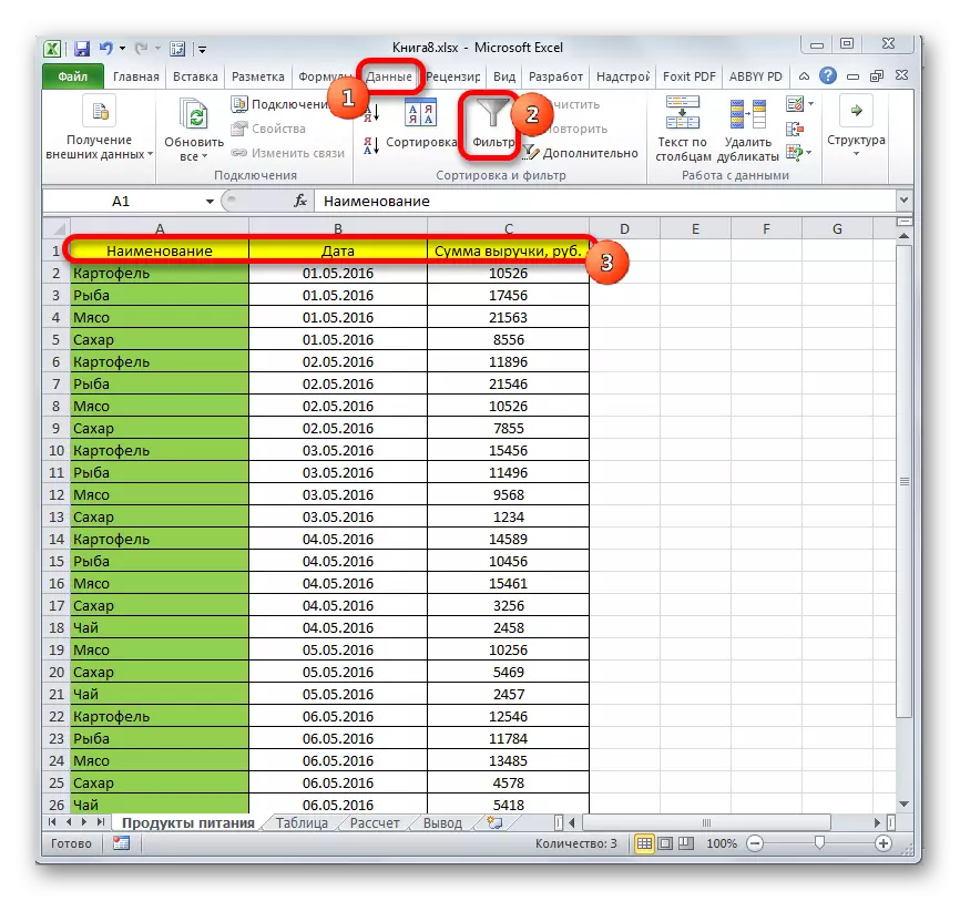
In order to hide the contents from the sheet, which will not need it in the near future so that it does not interfere, you can apply filtering.

1. We highlight the entire table or one of the cells in its cap. In the "Home" tab, click on the "Sort and Filter" icon, which is located in the Editing toolbar. A list of actions opens where you select the "Filter" item.

   

   You can also do otherwise. After selecting a table or caps, go to the Data tab. Clicks on the "Filter" button. It is located on the ribbon in the "Sort and Filter" block.



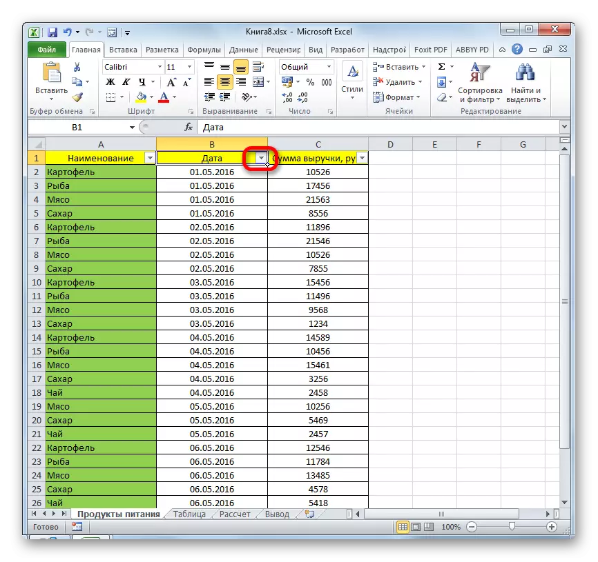
2. Whatever of the two proposed ways you do not use, the filtering icon will appear in the table cap cells. It is a small triangle of black color, directional angle down. Click on this icon in the column, where the sign is contained by which we will filter the data.



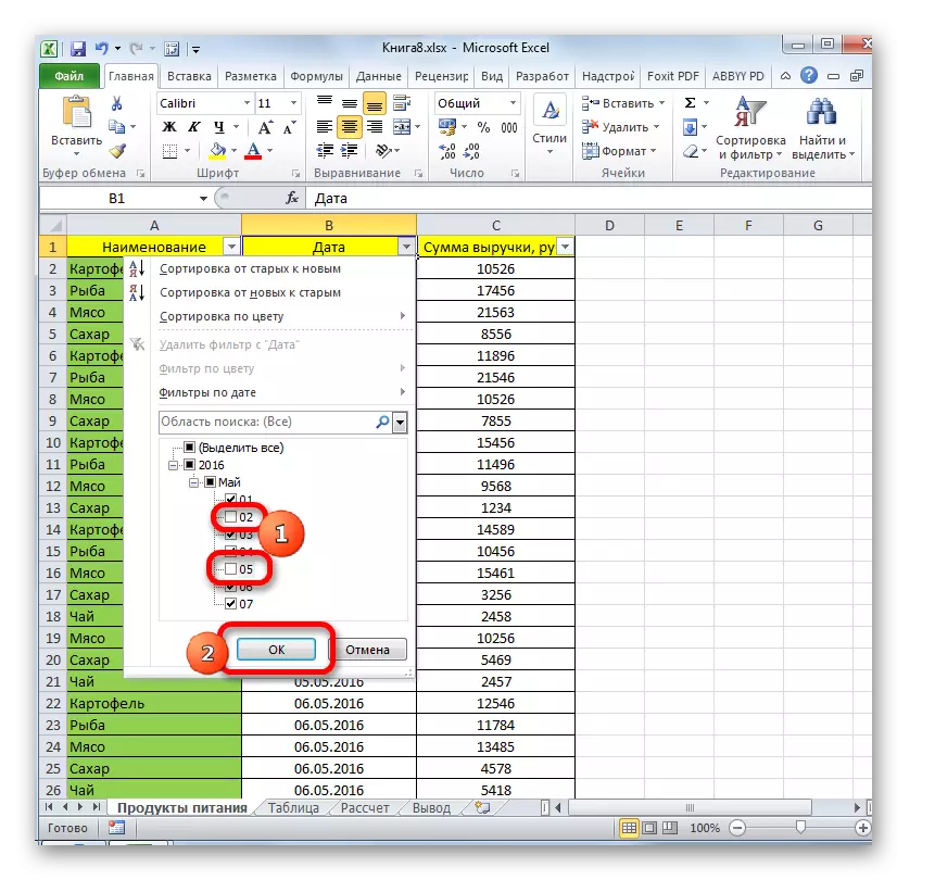
3. The filtering menu opens. Remove ticks from those values ​​that are contained in rows designed to hide. Then click on the "OK" button.



4. After this action, all the lines where there are values ​​from which we removed the checkboxes will be hidden using the filter.

Lesson: Sorting and filtering data to Excel

Method 7: Hide cells

Now let's talk about how to hide individual cells. Naturally, they cannot be completely removed, like lines or columns, as it will destroy the structure of the document, but still there is a way if it does not completely hide the elements themselves, then hide their contents.

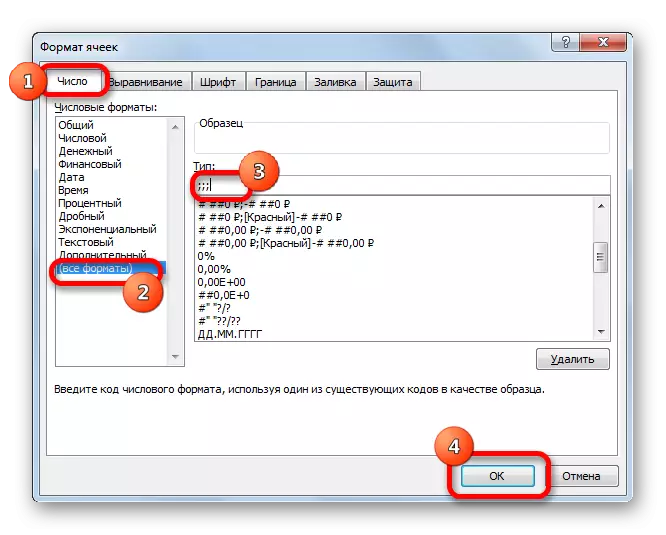
1. Select one or more cells to hide. Click on the dedicated fragment with the right mouse button. The context menu opens. Select it in it "Cell format ...".



2. The formatting window is launched. We need to go to his "Number" tab. Next, in the "Numeric formats" parameters, select the "All Formats" position. On the right side of the window in the "Type" field, drive the following expression:

   ;;;

   Click on the "OK" button to save the entered settings.



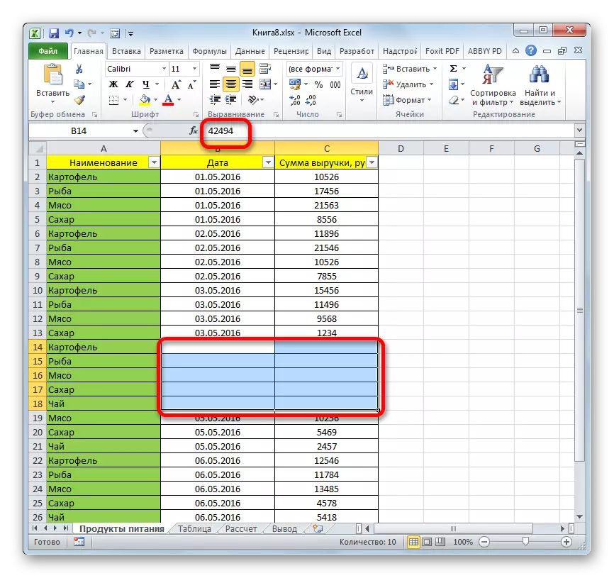
3. As you can see, after that, all data in the selected cells disappeared. But they disappeared only for the eyes, and in fact they continue to be there. To make sure this is enough to look at the string of the formulas in which they are displayed. If you need to turn on the display of data in the cells, you will need to change the format to the format in them through the format window.

As you can see, there are several different ways with which you can hide lines in Excel. Moreover, most of them use completely different technologies: filtering, grouping, shift boundaries of cells. Therefore, the user has a very wide selection of tools to solve the task. It can apply the option that considers more appropriate in a particular situation, as well as more comfortable and easy for himself. In addition, using formatting it is possible to hide the contents of individual cells.