

One of the basic economic and financial calculations of any enterprise is to define its break-even point. This indicator indicates that, with what volume of production, the organization's activities will be cost-effective and it will not suffer damages. The Excel program provides users with tools that greatly make it easier to define this indicator and display the result obtained graphically. Let's find out how to use them when you find a break-even point on a specific example.
Break even
The essence of the break-even point is to find the amount of production volume, in which the profit size (losses) will be zero. That is, with an increase in production volumes, the company will begin to show the profitability of activity, and with a decrease - unprofitability.When calculating the break-even point, it is necessary to understand that all costs of the enterprise can be divided into permanent and variables. The first group does not depend on the volume of production and is constant. This can include the volume of wages to administrative staff, the cost of renting premises, depreciation of fixed assets, etc. But variable costs are directly dependent on the volume of products produced. This, first of all, should include costs for the acquisition of raw materials and energy carriers, therefore this type of costs are taken to indicate a unit of manufactured products.
It is with the ratio of constant and variable costs that the concept of break-even point is associated. Prior to the achievement of a certain amount of production, constant costs are a significant amount in the total cost of products, but with an increase in the volume of their share falls, which means that the cost of the unit produced is falling. At the level of break-even point, the cost of production and income from the sale of goods or services is equal. With a further increase in production, the company begins to make a profit. That's why it is so important to determine the volume of production at which the break-even point is achieved.
Calculation of break-even point
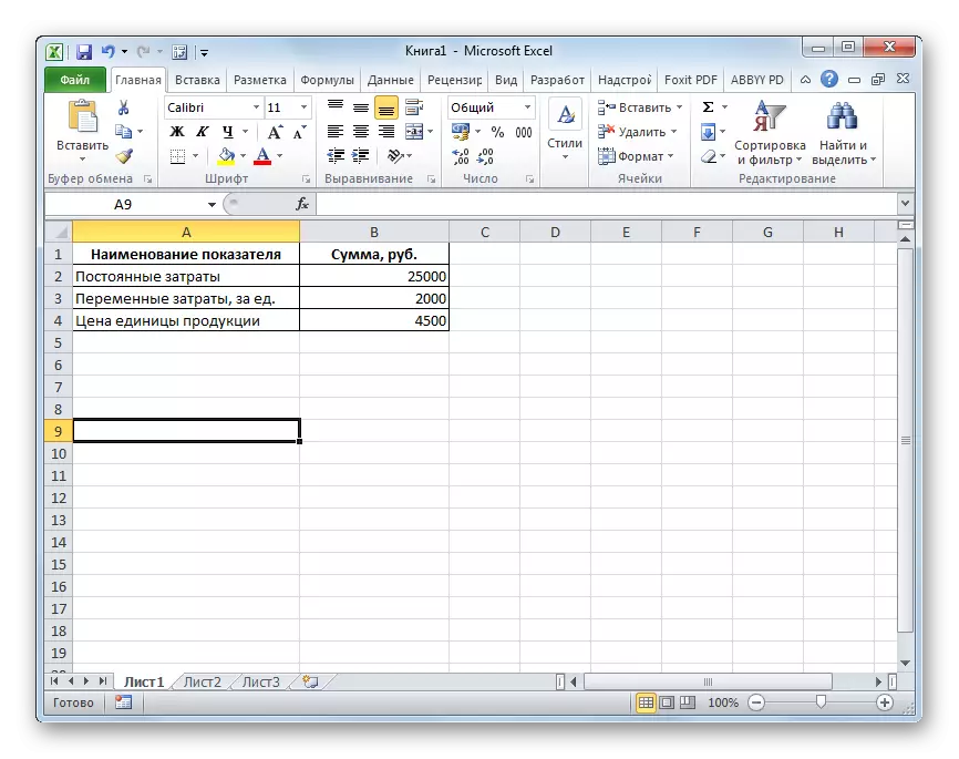
Calculate this indicator using the Excel program tools, as well as build a graph where you will mention the break-even point. To carry out calculations, we will use the table in which such initial data of the enterprise are indicated:
- Constant costs;
- Variable costs per unit of production;
- Price implementation of products.
So, we will calculate data based on the values specified in the table in the image below.
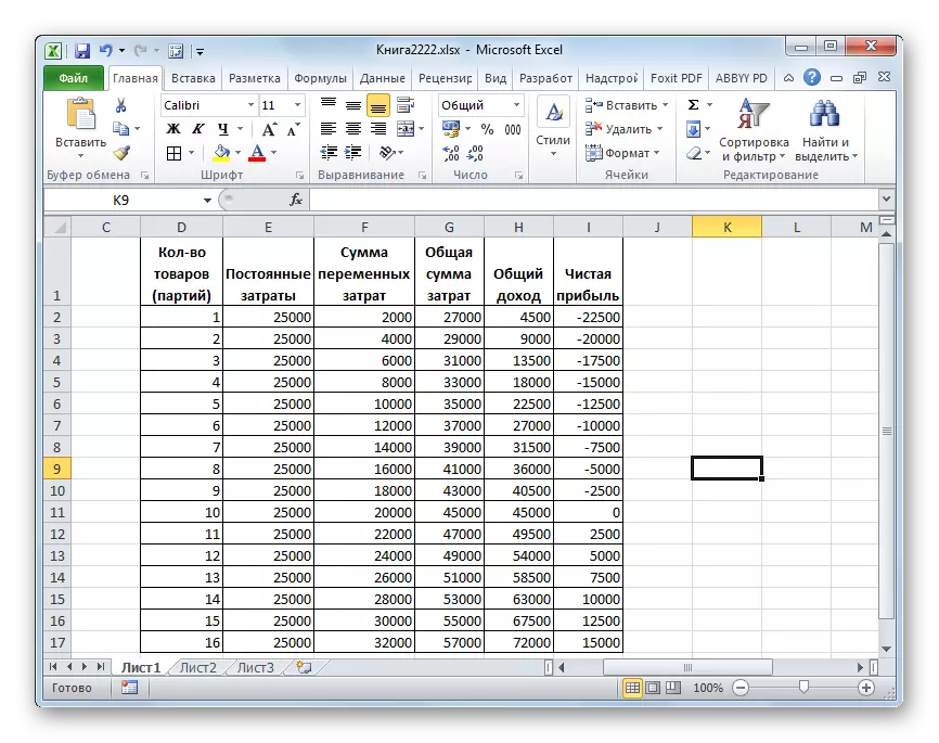
- Build a new table based on the source table. The first column of the new table is the amount of goods (or parties) manufactured by the enterprise. That is, the line number will indicate the amount of manufactured goods. In the second column there is a magnitude of constant costs. It will be 25,000 in our lines in all rows. In the third column - the total amount of variable costs. This value for each row will be equal to the product number of goods, that is, the contents of the corresponding cell of the first column, for 2000 rubles.
In the fourth column there is a total amount of expenses. It is the sum of the cells of the corresponding line of the second and third column. In the fifth column there is a total income. It is calculated by multiplying the price of a unit of goods (4500 p.) To the aggregate amount, which is indicated in the corresponding line of the first column. In the sixth column there is a net profit indicator. It is calculated by subtracting from the overall income (column 5) cost amounts (column 4).
That is, in those lines that in the respective cells of the last column will be a negative value, the enterprise loss is observed, in those where the indicator will be 0 - the break-even point has been reached, and in those where it will be positive - the profit is marked in the organization's activities.
For clarity, fill 16 lines. The first column will be the number of goods (or parties) from 1 to 16. Subsequent columns are filled in by the algorithm that was listed above.
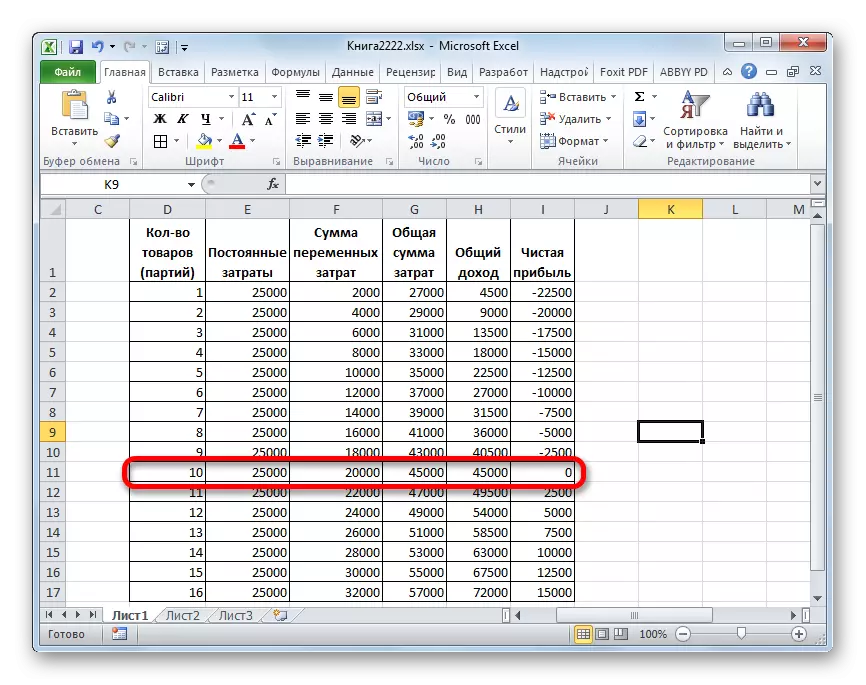
- As you can see, the break-even point is reached on the 10 product. It was then that the total income (45,000 rubles) is equal to cumulative expenses, and net profit is 0. Already starting with the release of eleventh goods, the company shows profitable activities. So, in our case, the break-even point in the quantitative indicator is 10 units, and in the money - 45,000 rubles.
Creating a graph
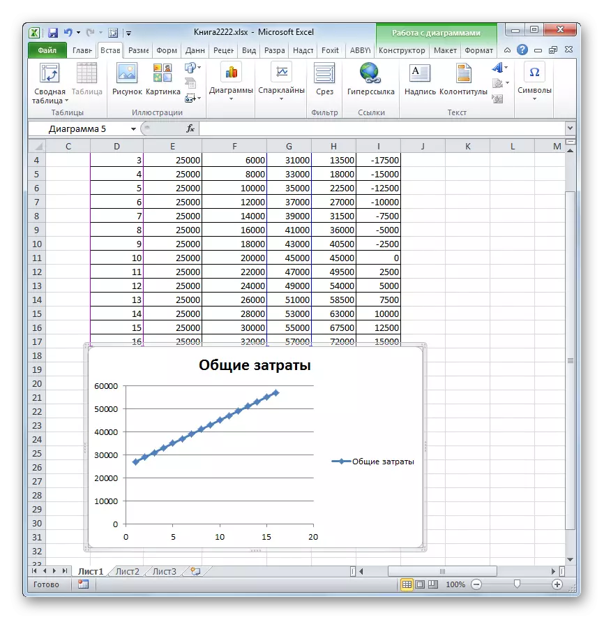
After the table was created in which the break-even point is calculated, you can create a chart where this pattern will be displayed visually. To do this, we will have to build a diagram with two lines that reflect the costs and income of the enterprise. At the intersection of these two lines and there will be a break-even point. On the x axis of this diagram, the number of goods will be located, and in the Y axis y threads.
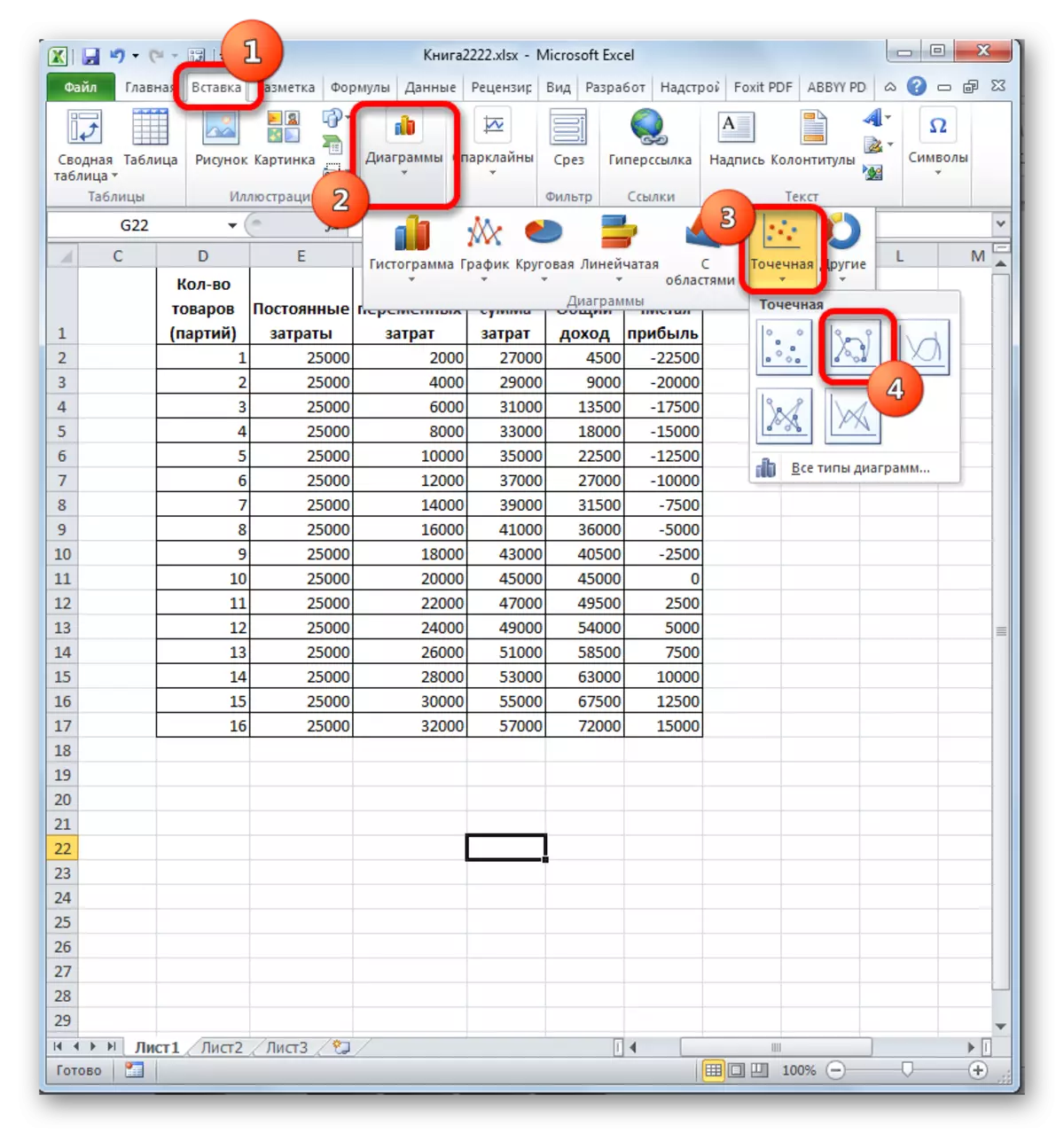
- Go to the "Insert" tab. Click on the "Spot" icon, which is placed on the tape in the "Chart toolbar" block. We have a choice of several types of graphs. To solve our problem, the type "Spotted with smooth curves and markers" is quite suitable, so click on this element of the list. Although, if you wish, you can use some other types of diagrams.
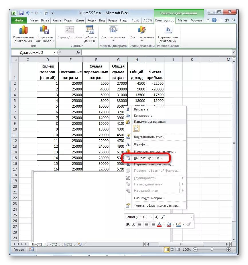
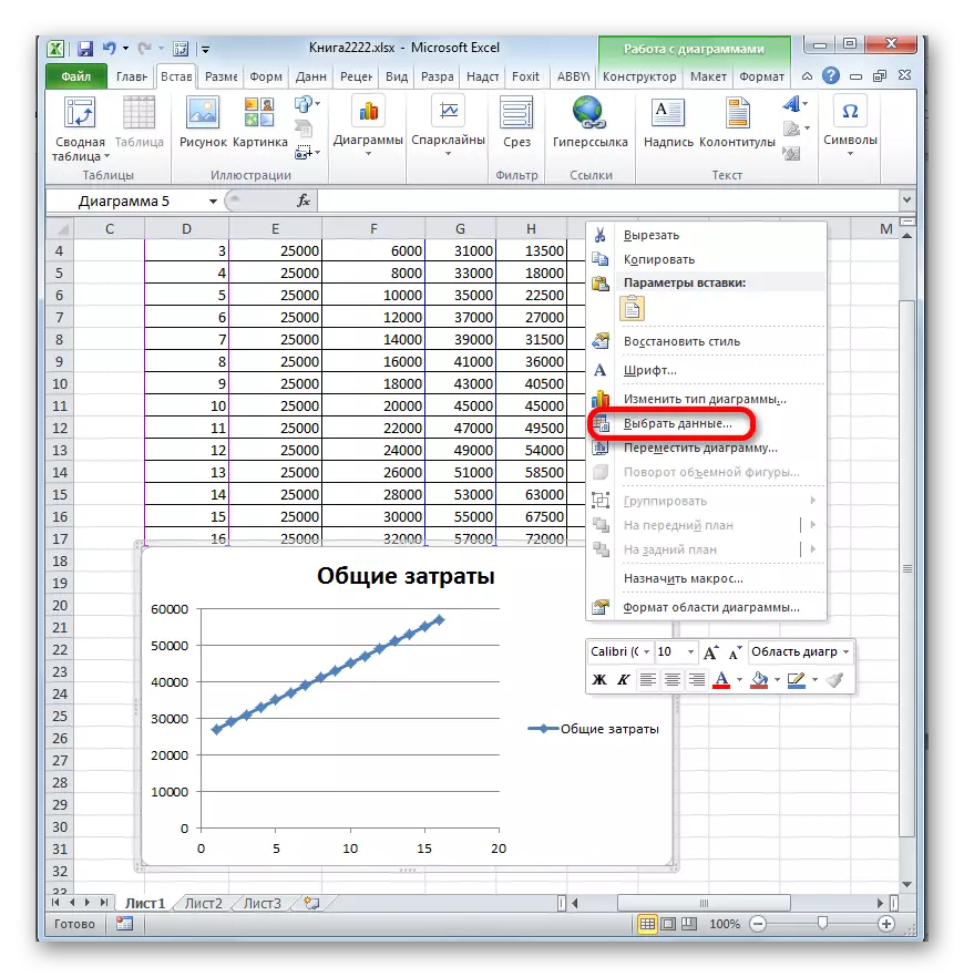
- Before us opens an empty area of the chart. You should fill it with data. To do this, click the right mouse button around the area. In the activated menu, select the "Select data ..." position.
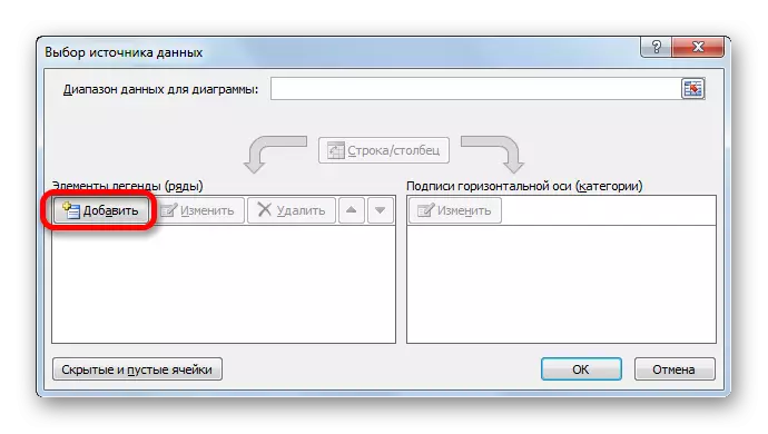
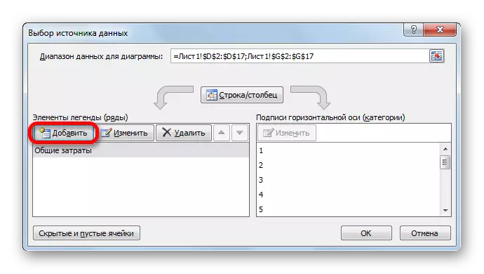
- The data source selection window is launched. In his left part there is a block "elements of legends (ranks)". Click on the "Add" button, which is placed in the specified block.
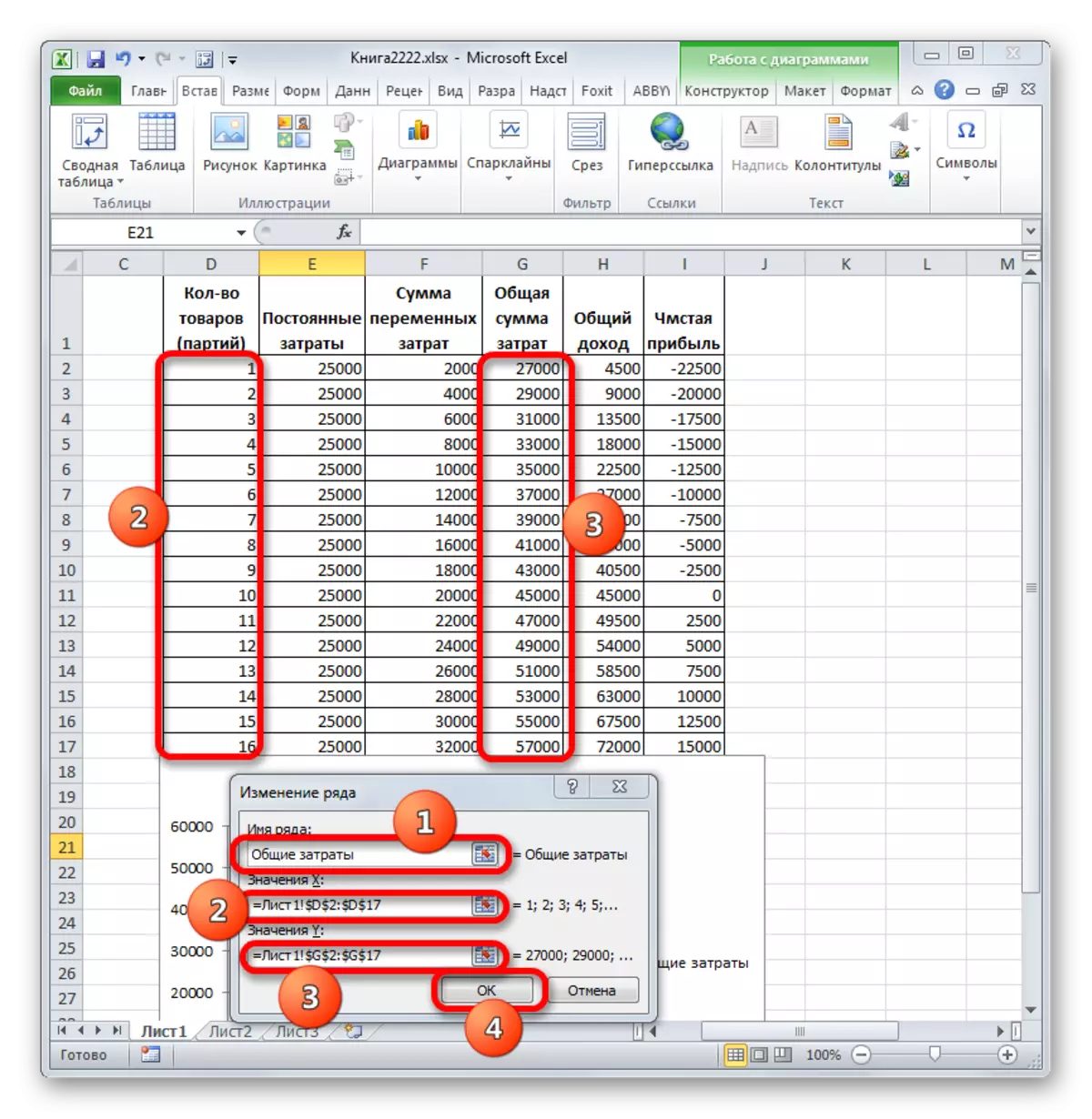
- We have a window called "Changing a Row". In it, we must specify the coordinates of the placement of data on which one of the graphs will be built. To begin with, we will build a schedule in which the total costs would be displayed. Therefore, in the "Row Name" field, you enter the "General Costs" recording from the keyboard.
In the "X Value" field, specify the data coordinates located in the "Number of Goods" column. To do this, set the cursor in this field, and then by producing the clip of the left mouse button, select the corresponding column of the table on the sheet. As we can see, after these actions, its coordinates will be displayed in the window of changing the row.
In the following field "V values", display the "Total Costs" column address, in which the data we need are located. We act on the above algorithm: we put the cursor in the field and highlight the cells of the column we need with the left-click of the mouse. Data will be displayed in the field.
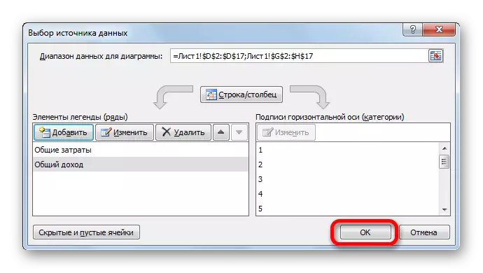
After the specified manipulations were carried out, click on the "OK" button, placed in the lower part of the window.
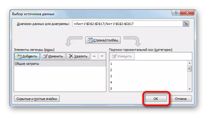
- After that, it automatically returns to the data source selection window. It also needs to click on the "OK" button.
- As you can see, following this, a schedule of the total cost of the enterprise will appear on the sheet.
- Now we have to build a line of general income of the enterprise. For these purposes, with the right mouse button on the diagram area, which already contains the line of the total cost of the organization. In the context menu, select the "Select data ..." position.
- A window for selecting a source of data in which again you want to click on the Add button again.
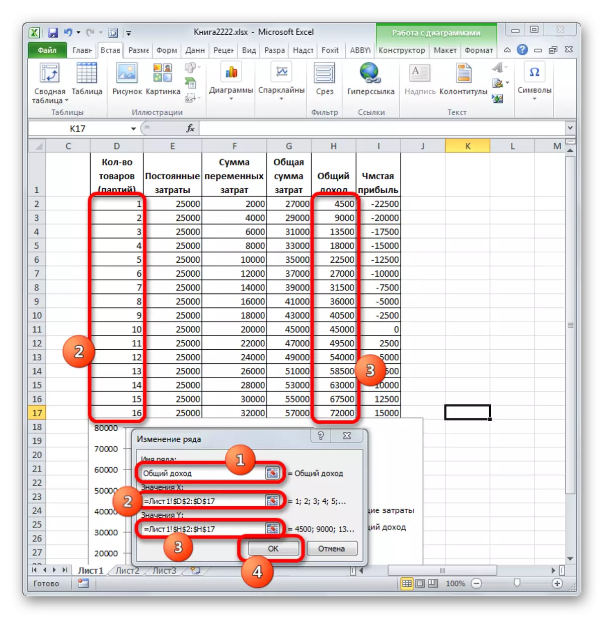
- A small window of changing a series opens. In the "Row name" field this time we write "Common Income".
In the "Value X" field, the coordinates of the column "The number of goods" should be made. We do this in the same way that we considered when building a line of total costs.
In the "V values" field, exactly indicate the coordinates of the "Total Income" column.
After performing these actions, we click on the "OK" button.
- Close source selection window by pressing the "OK" button.
- After that, the general income line will appear on the sheet plane. It is the point of intersection of general income lines and total costs will be a break-even point.
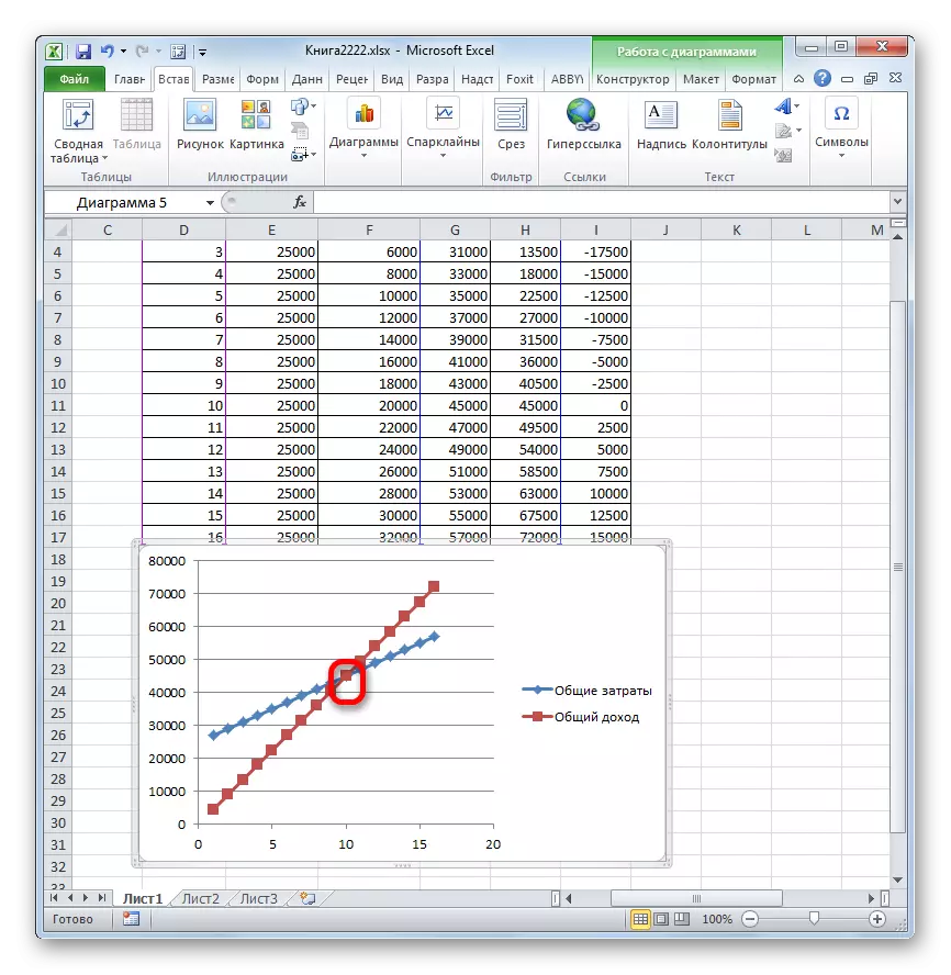
Thus, we have achieved the objectives of creating this schedule.
Lesson: How to make a chart in exile
As you can see, finding a break-even point is based on the determination of the amount of products produced, in which the total costs will be equal to general income. This is graphically reflected in the construction of costs and income lines, and in finding the point of their intersection, which will be a break-even point. Conducting such calculations is the basic in organizing and planning the activities of any enterprise.