Calculation of annuity pay in Excel

Before taking the loan, it would be nice to calculate all payments on it. It will save the borrower in the future from various unexpected troubles and disappointments when it turns out that overpayment is too big. Help on this calculation can the Excel program tools. Let's find out how to calculate the annuity payments on the loan in this program.

Calculation of payment

First of all, it must be said that there are two types of credit payments:

• Differentiated;
• Annuity.

With a differentiated scheme, the client brings a monthly equal share of payments on the body of a loan plus payments to interest. The magnitude of interest payments each month decreases, as the body of the loan is reduced from which they are calculated. Thus, the overall monthly payment is also reduced.

Ann aunt scheme uses a slightly different approach. The client makes a single amount of the total payment monthly, which consists of payments on the body of a loan and payment of interest. Initially, interest contributions are numbered on the entire amount of the loan, but as the body decreases, interest is reduced and interest accrual. But the total amount of payment remains unchanged due to a monthly increase in the amount of payments by the body of the loan. Thus, over time, the proportion of interest in the total monthly payment falls, and the proportion weight of the body grows. At the same time, the general monthly payment itself is not changing throughout the term of credit.

Just on the calculation of the annuity payment, we will stop. Especially, this is relevant, since now most banks use this particular scheme. It is convenient for customers, because in this case the total amount of payment does not change, remaining fixed. Customers always know how much you need to pay.

Step 1: Monthly Contribution Calculation

To calculate a monthly contribution when using an annuity circuit in Excele, there is a special function - PPT. It refers to the category of financial operators. The formula of this feature is as follows:

= PPT (rate; KPER; PS; BS; type)

As we see, the specified function has a fairly large number of arguments. True, the last two of them are not mandatory.

The "rate" argument indicates a percentage rate for a specific period. If, for example, an annual rate is used, but the loan payment is made monthly, then the annual rate must be divided into 12 and the result is used as an argument. If a quarterly type of payment is applied, then in this case the annual bet must be divided into 4, etc.

"Cper" means the total number of periods of loan payments. That is, if the loan is taken for one year with the monthly payment, then the number of periods is considered 12, if two years, then the number of periods - 24. If the loan is taken for two years with quarterly payment, then the number of periods is 8.

"PS" indicates the present value at the moment. Speaking with simple words, this is the total amount of the loan at the beginning of lending, that is, the amount you are borrowed, excluding interest and other additional payments.

"BS" is a future cost. This value will be a loan body at the time of completion of the loan agreement. In most cases, this argument is "0", since the borrower at the end of the credit period should fully settle with the lender. The specified argument is not mandatory. Therefore, if it is descended, it is considered to be zero.

The "Type" argument determines the calculation time: at the end or at the beginning of the period. In the first case, it takes the value "0", and in the second - "1". Most banking institutions use exactly the option with payment at the end of the period. This argument is also optional, and if it is omitted, it is believed that it is zero.

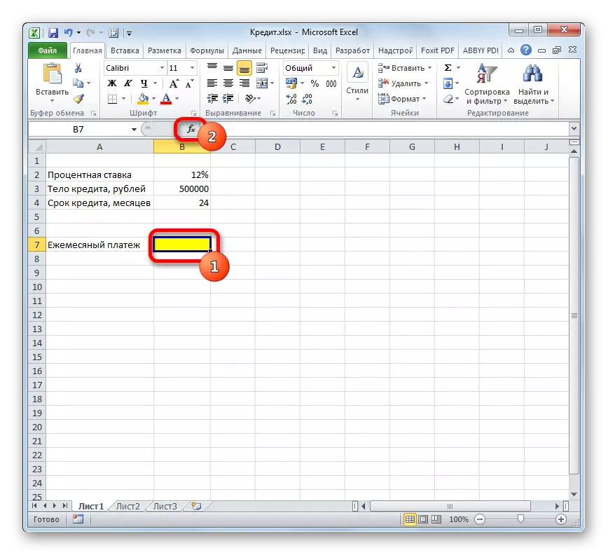
Now it is time to move to a specific example of calculating a monthly contribution using the PL function. To calculate, we use a table with the source data, where the interest rate on the loan (12%) is indicated, the loan value (500,000 rubles) and the loan period (24 months). At the same time, payment is made monthly at the end of each period.

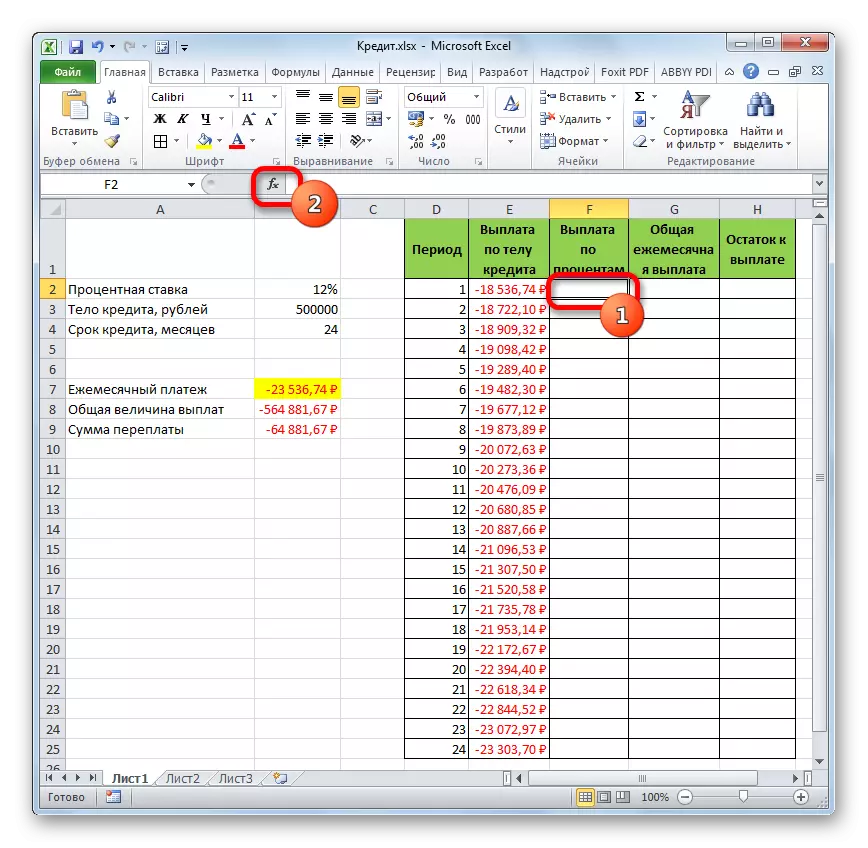
1. Select the element on the sheet into which the result result will be displayed, and click the "Insert function" icon, placed near the formula row.



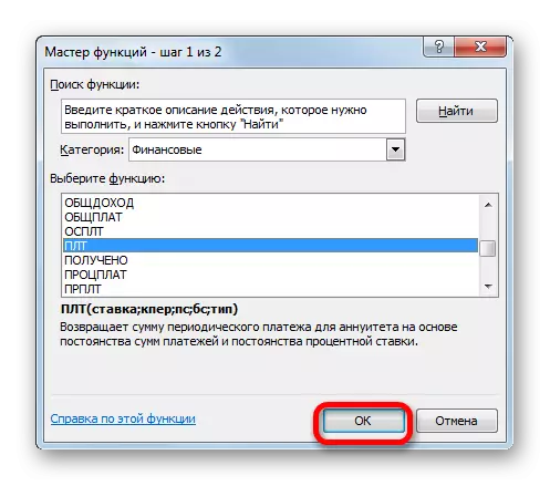
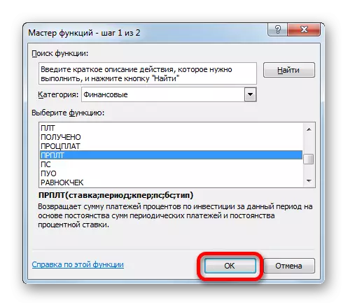
2. The window wizard window is launched. In the category "Financial" allocate the name "PLT" and click on the "OK" button.



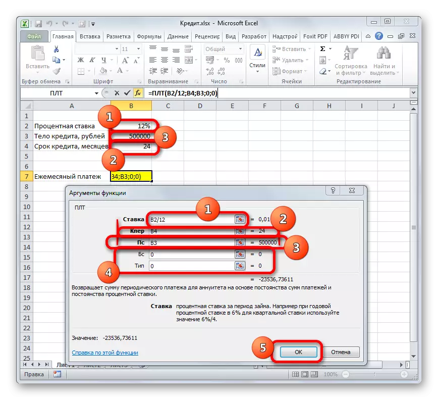
3. After that, opens the arguments window of the PL operator.

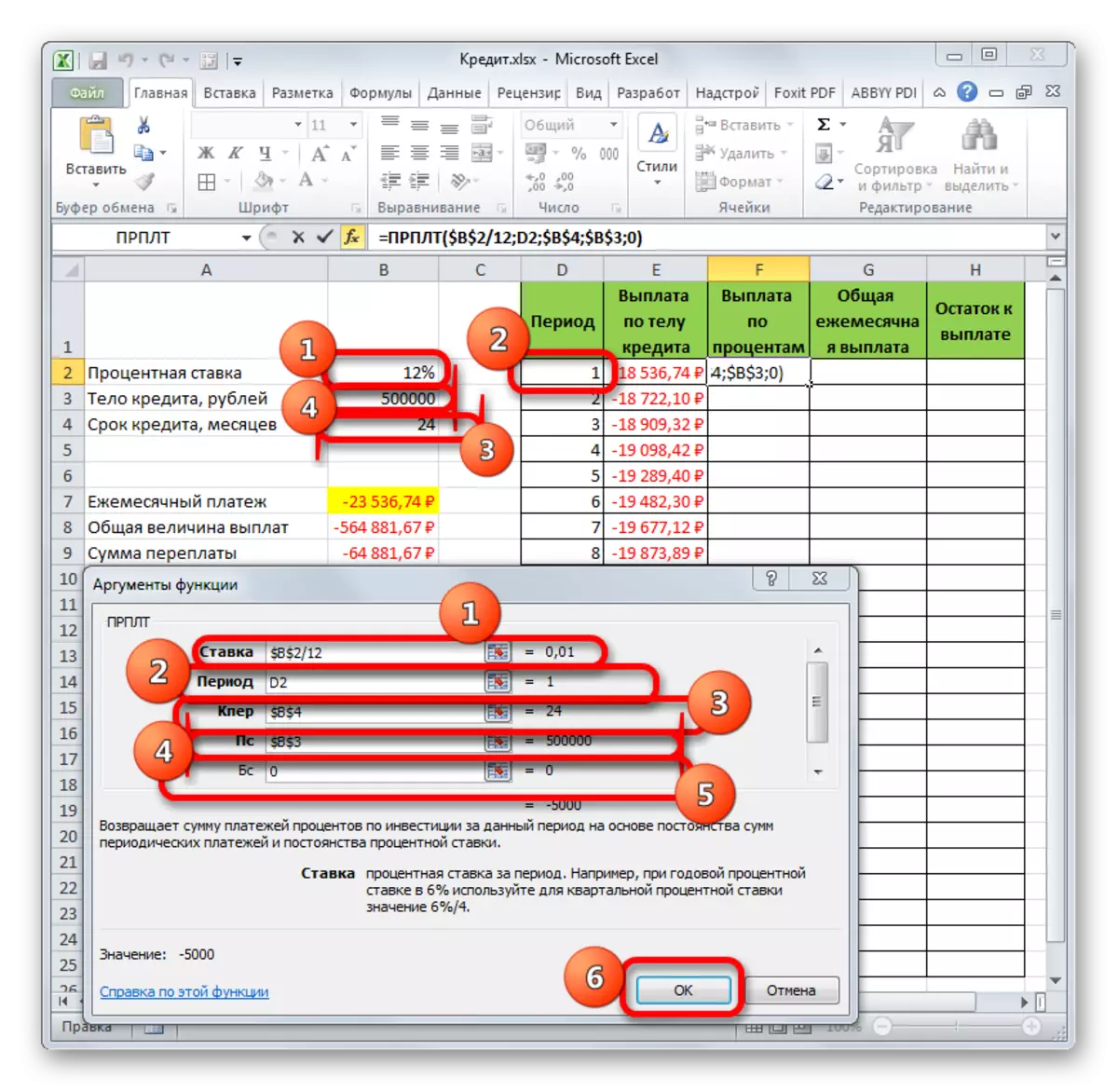
   In the "Rate" field, you should enter the percentage value for the period. This can be done manually, just putting a percentage, but it is indicated in a separate cell on the sheet, so we will give a link to it. Install the cursor in the field, and then click on the corresponding cell. But, as we remember, we have the annual interest rate in our table, and the payment period is equal to the month. Therefore, we divide the annual bet, and rather a link to the cell in which it is contained by the number 12, corresponding to the number of months in the year. Division run directly in the Argument window field.

   In the Cper field, lending is set. He is equal to 24 months. You can apply in the number 24 manually field, but we, as in the previous case, specify a link to the location of this indicator in the source table.

   In the field "PS" indicates the initial loan value. It is equal to 500,000 rubles. As in the previous cases, we specify a link to the leaf element, which contains this indicator.

   In the field "BS" indicates the magnitude of the loan, after its full payment. As you remember, this value is almost always zero. Install in this field the number "0". Although this argument can generally be omitted.

   In the "Type" field, we specify at the beginning or at the end of the month payment is made. We, as in most cases, it is produced at the end of the month. Therefore, we set the number "0". As in the case of the previous argument, it is possible to enter anything to this field, then the default program will assume that it is zero equal to it.

   After all the data is entered, press the "OK" button.



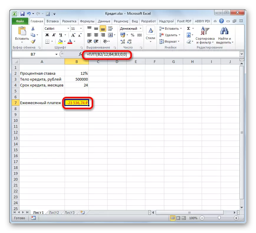
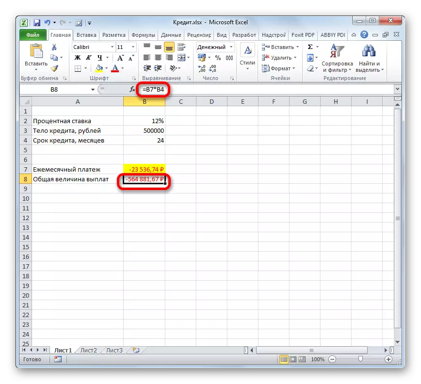
4. After that, in the cell that we allocated in the first paragraph of this manual, the result of the calculation is displayed. As you can see, the magnitude of the monthly general payment on the loan is 23536.74 rubles. Let you not confuse the sign "-" before this amount. So Exile indicates that this is the flow of money, that is, a loss.



5. In order to calculate the total amount of payment for the entire loan period, taking into account the repayment of the body of a loan and monthly interest, rather multiply the amount of the monthly payment (23536.74 rubles) for the number of months (24 months). As you can see, the total amount of payments for the entire loan period in our case was 564881.67 rubles.



6. Now you can calculate the amount of loan overpayment. To do this, it is necessary to take away from the total amount of payments on the loan, including interest and the loan body, the initial amount claimed. But we remember that the first of these values ​​already with the sign "-". Therefore, in specifically, our case it turns out that they need to be folded. As we see, the total overpayment of the loan over the entire period was 64881.67 rubles.

Lesson: Master of Functions in Excel

Stage 2: Payment Details

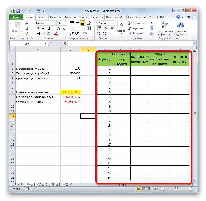
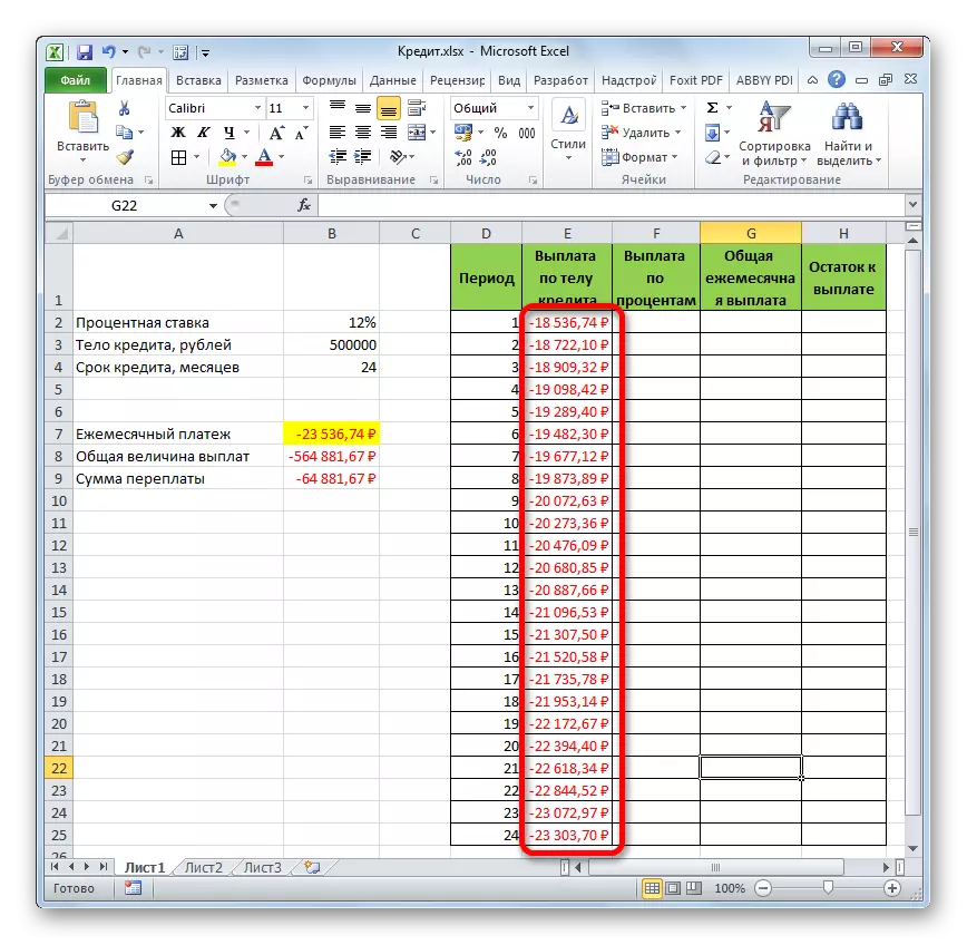
And now, with the help of other Excel operators, we make a monthly detail of payments to see how much in a specific month we pay through the body of the loan, and how much is the amount of interest. For these purposes, blacksmith in the exile table, which we will fill in the data. The lines of this table will be responsible to the corresponding period, that is, the month. Given that the period of lending is 24 months, the number of rows will also be appropriate. The columns indicated a loan body, interest payments, a total monthly payment, which is the sum of the previous two columns, as well as the remaining amount to pay.

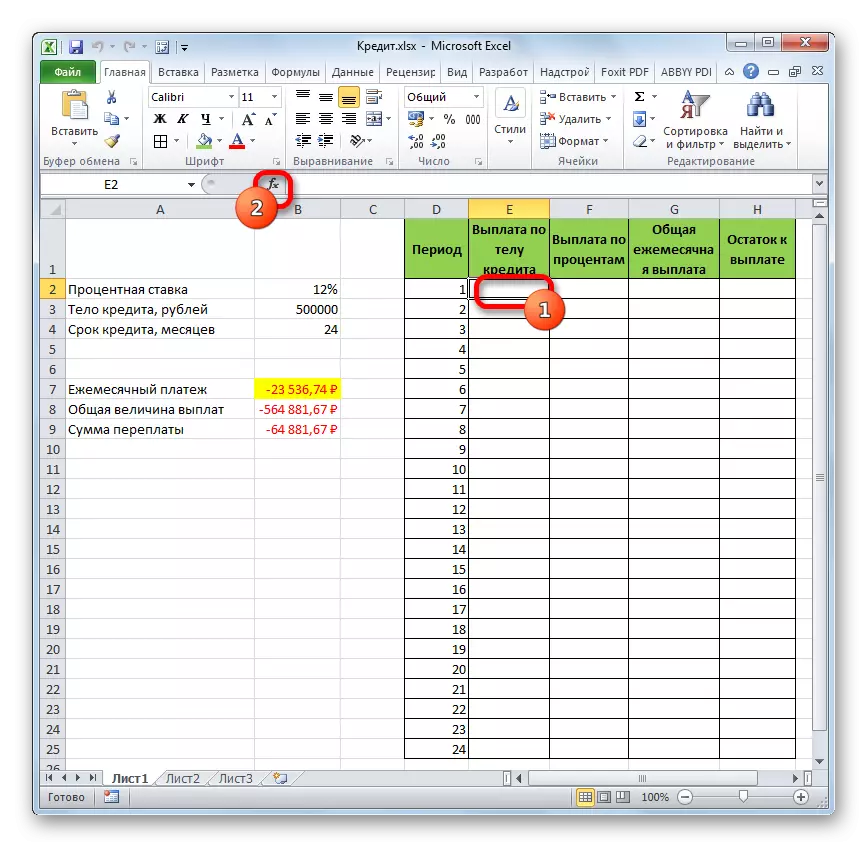
1. To determine the amount of payment by the body of the loan, use the OSP function, which is just intended for these purposes. We establish the cursor in the cell, which is located in the line "1" and in the column "Payment by the body of the loan". Click on the "Paste Function" button.



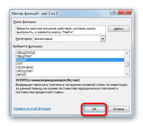
2. Go to the Master of Functions. In the category "Financial", we note the name "OSPLT" and click the "OK" button.



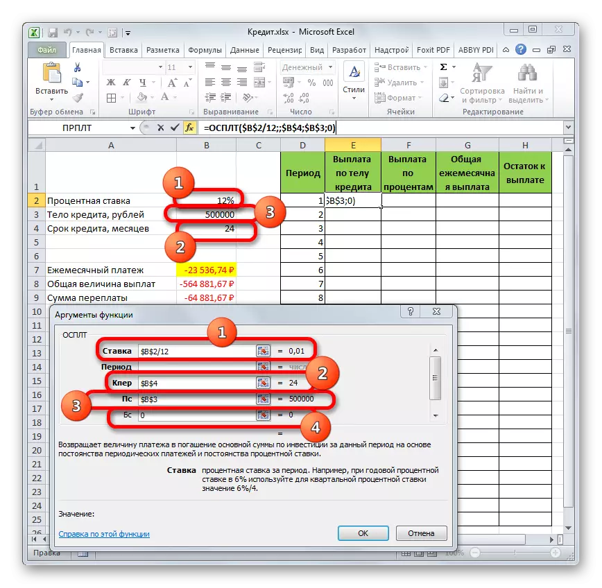
3. The arguments of the OSP operator arguments start. It has the following syntax:

   = Ospult (rate; period; KPER; PS; BS)

   As we can see, the arguments of this feature almost completely coincide with the arguments of the PLT operator, only instead of the optional argument "Type" added a mandatory argument "period". It indicates the number of the payment period, and in our particular case on the number of the month.

   Fill out the arguments of the OSR function arguments already familiar to us by the same data, which was used for the PL function. Just given the fact that in the future, copying a formula will be used through a filling marker, you need to do all links in the fields absolute so that they do not change. This requires to put a dollar sign before each value of vertical and horizontal coordinates. But it is easier to do it, simply selecting the coordinates and clicking on the F4 function key. The dollar sign will be placed in the right places automatically. We also do not forget that the annual bet must be divided into 12.



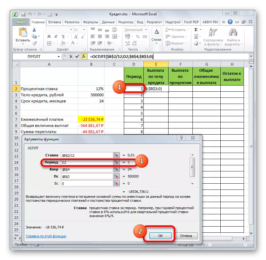
4. But we have another new argument, which was not from the PL function. This argument "period". In the appropriate field, set a reference to the first cell of the "period" column. This element of the sheet contains the number "1", which denotes the number of the first month of lending. But unlike the previous fields, we leave the link relative in the specified field, and not do absolute from it.

   After all the data about which we talked above are introduced, press the "OK" button.



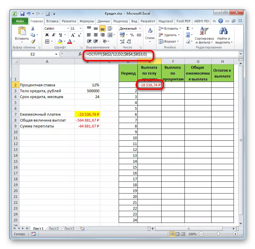
5. After that, in the cell, which we previously allocated, the amount of payment by the body of the loan for the first month will appear. It will be 18536.74 rubles.



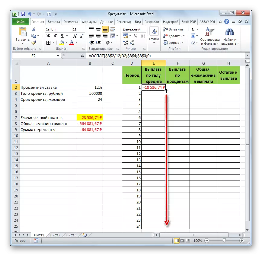
6. Then, as mentioned above, we should copy this formula to the remaining column cells using a filling marker. To do this, set the cursor to the lower right corner of the cell, which contains the formula. The cursor is converted to a cross, which is called a filling marker. Click the left mouse button and pull it down to the end of the table.



7. As a result, all cell columns are filled. Now we have a chart of paying a loan monthly. As mentioned above, the amount of payment on this article increases with each new period.



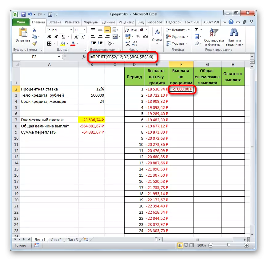
8. Now we need to make a monthly payment calculation by interest. For these purposes, we will use the PRT operator. We allocate the first empty cell in the "Payments percentage" column. Click on the "Paste Function" button.



9. In the functions of the Master of Functions in the "Financial" category, we produce the names of the NAMP. Perform a click on the "OK" button.



10. The arguments window of the TRP function starts. Its syntax looks like this:

    = PRT (rate; period; CPU; PS; BS)

    As we can see, the arguments of this function are absolutely identical to similar elements of the OSP operator. Therefore, just enter the same data into the window that we entered in the previous window of the arguments. We do not forget that the reference in the "period" field should be relative, and in all other fields the coordinates should be brought to the absolute form. After that, click on the "OK" button.



11. Then the result of calculating the amount of payment for interest for a loan for the first month is displayed in the corresponding cell.



12. Applying the filling marker, make copying of the formula into the remaining elements of the column, in this way receiving a monthly schedule for percentages for the loan. As we can see, as it was said earlier, from month to month the value of this type of payment decreases.



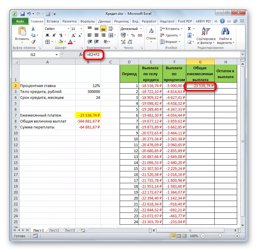
13. Now we have to calculate the overall monthly payment. For this calculation, one should not resort to any operator, as you can use the simple arithmetic formula. We fold the contents of the cells of the first month of the columns "Payment by the body of the loan" and "Full interest". To do this, set the sign "=" into the first empty cell of the column "total monthly payment". Then click on the two above elements by setting the "+" sign between them. Click on the ENTER key.



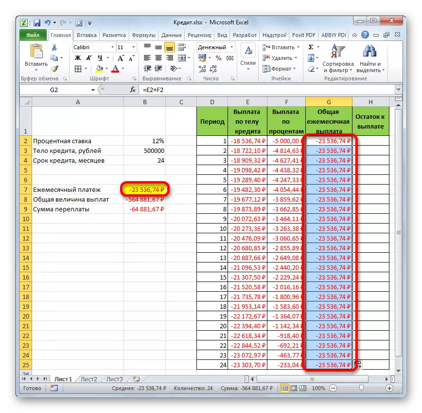
14. Next, using the filling marker, as in the previous cases, fill in the data column. As we can see, throughout the entire action of the contract, the amount of the total monthly payment, which includes payment by the body of the loan and payment of interest, will be 23536.74 rubles. Actually, we already calculated this indicator before using PPT. But in this case it is presented more clearly, precisely as the amount of payment by the body of the loan and interest.



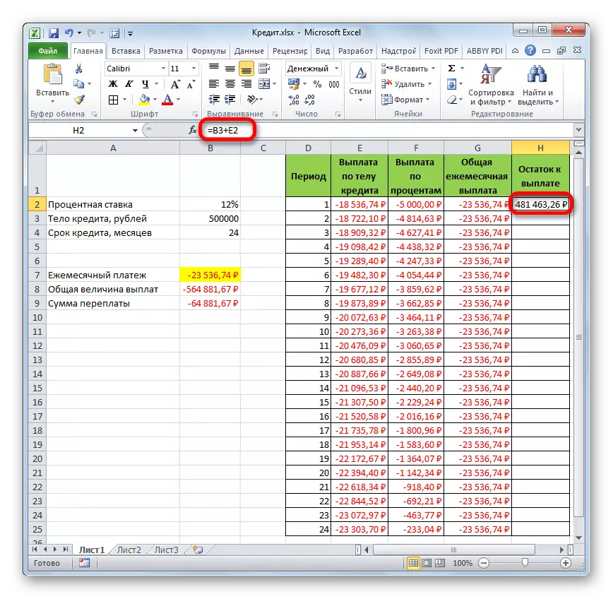
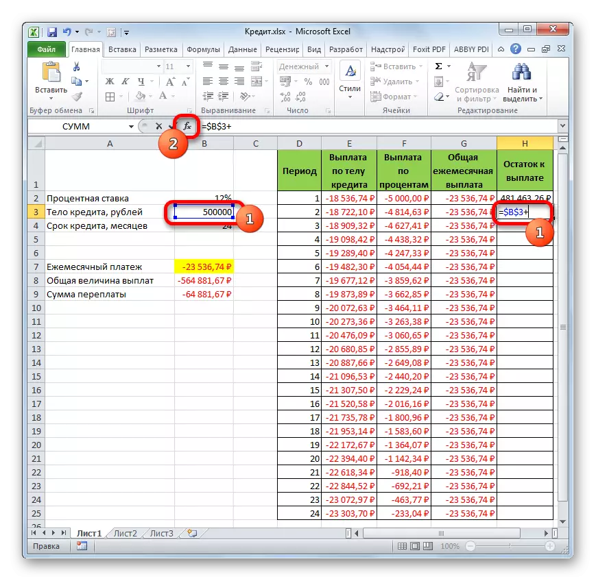
15. Now you need to add data to the column, where the balance of the loan amount is displayed monthly, which is still required to pay. In the first cell of the column "Balance to Pay" the calculation will be the easiest. We need to be taken away from the initial loan magnitude, which is specified in the table with primary data, the payment by the body of the loan for the first month in the calculated table. But, given the fact that one of the numbers we already go with the sign "-", then they should not be taken away, but to fold. We make it and click on the ENTER button.



16. But the calculation of the balance to pay after the second and subsequent months will be somewhat more complicated. To do this, we need to take away from the body of the loan to the beginning of lending the total amount of payments by the body of the loan for the previous period. Install the "=" sign in the second cell of the Column "Palace to Pay". Next, specify a link to the cell, which contains the initial loan amount. We make it absolute, highlighting and pressing the F4 key. Then we put the sign "+", since we have the second meaning and so negative. After that, click on the "Insert function" button.



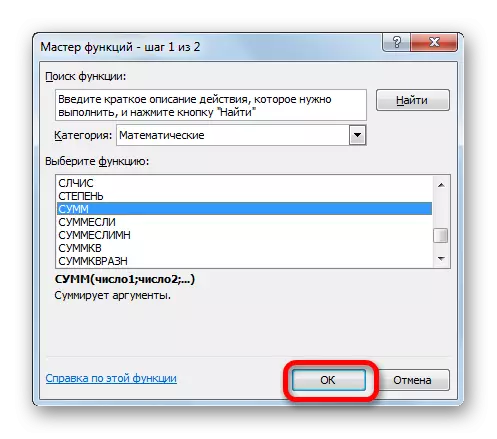
17. The master of functions is launched, in which you need to move to the category "Mathematical". There we allocate the inscription "sums" and press the "OK" button.



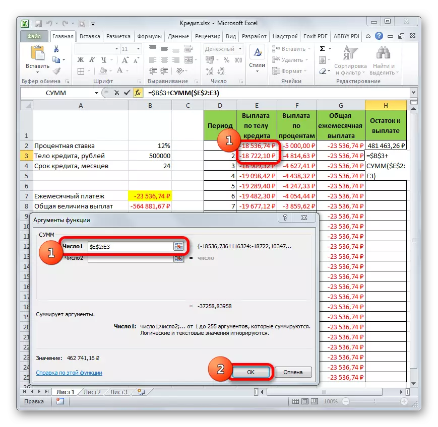
18. The arguments window starts the function arguments. The specified operator serves to summarize the data in the cells that we need to perform in the "Payment by the Loan Body" column. It has the following syntax:

    = Sums (number1; number2; ...)

    As arguments, references to cells in which numbers are contained. We set the cursor in the "Number1" field. Then pin the left mouse button and select the first two cells of the Credit Body column on the sheet. In the field, as we see, a link to the range appeared. It consists of two parts separated by the colon: references to the first range of the range and on the last one. In order to be able to copy the specified formula in the future by a filling marker, we make the first link to the absolute range. We highlight it and click on the F4 function key. The second part of the reference and leave relative. Now, when using a filling marker, the first range of the range will be fixed, and the latter will stretch as it moves downwards. This is necessary for us to fulfill the goals. Next, click on the "OK" button.



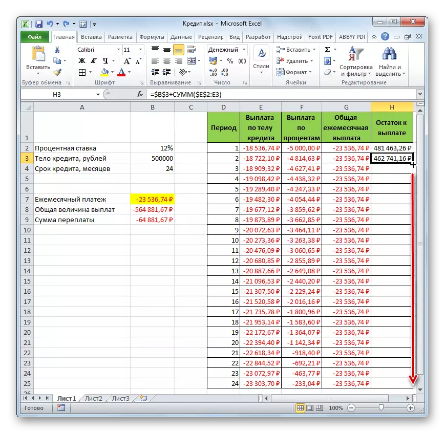
19. So, the result of the balance of credit debt after the second month is discharged into the cell. Now, starting with this cell, we make copying the formula into empty column elements using a filling marker.



20. Monthly calculation of remnants to pay on the loan is made for the entire credit period. As it should be, at the end of the deadline, this amount is zero.

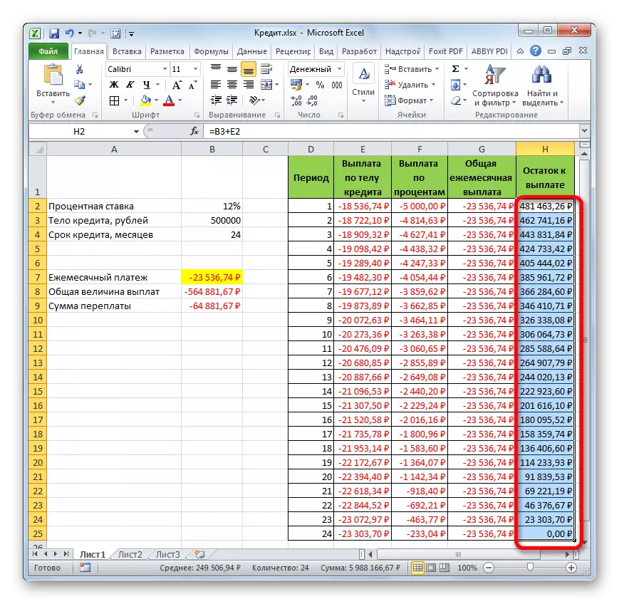
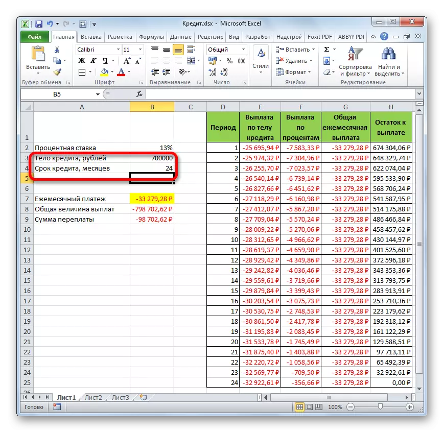
Thus, we did not simply calculate the loan payment, but organized a kind of credit calculator. Which will act on an annuity scheme. If in the source table we, for example, change the amount of the loan and the annual interest rate, then in the final table there will be automatic data recalculation. Therefore, it can be used not only once for a particular case, but to apply in various situations to calculate credit options on an annuity scheme.

Lesson: Financial functions in Excel

As you can see, using the Excel program at home, you can easily calculate the overall monthly loan payment on the annuity scheme, using the PL operator for these purposes. In addition, with the help of OSR functions and the PRT, it is possible to calculate the amount of payments by the body of the loan and percentages for the specified period. Applying all this luggage functions together, it is possible to create a powerful credit calculator that can be used more than once to calculate the annuity payment.