Function Four Excel

One of the embedded functions of the Excel program is dwarps. Its task is to return to the leaf element, where it is located, the contents of the cell on which the link in the text format is specified in the form of an argument.

It would seem that there is nothing special about it, since it is possible to display the contents of one cell in another and easier ways. But, as it turns out, some nuances that make it unique are associated with the use of this operator. In some cases, this formula is able to solve such tasks with which in other ways it simply cannot cope or it will be much more difficult to do. Let's learn more, which represents the Far operator and how it can be used in practice.

The use of Formula DVSSL

The very name of this operator DVSSL is decrypted as a "double link". Actually, this indicates its purpose - to display data through the specified reference from one cell to another. Moreover, unlike most other functions working with references, it must be specified in text format, that is, highlighted from both sides with quotes.

This operator refers to the category of "Links and arrays" functions and has the following syntax:

= Dwarf (link_namechair; [A1])

Thus, the formula has only two arguments.

The argument "Link to the cell" is presented as a link to the leaf element, the data contained in which you want to display. In this case, the specified link must have a text form, that is, being "wrapped" with quotes.

The argument "A1" is not mandatory and in the overwhelming majority of cases does not need to be indicated at all. It can have two values ​​of "Truth" and "Lie". In the first case, the operator determines the links in the style of "A1", namely, this style is enabled in Excel by default. If the value of the argument does not specify at all, it will be considered precisely as "truth". In the second case, references are determined in the style of R1C1. This link style must be specifically included in the EXEL settings.

If you say simply, the dwarf is a kind of equivalent of the links of one cell to another after the sign "equal." For example, in most cases an expression

= Dwarns ("A1")

will be equivalent to expression

= A1.

But in contrast to the expression "= A1", the operator DVSLs is attached not to a specific cell, but to the coordinates of the element on the sheet.

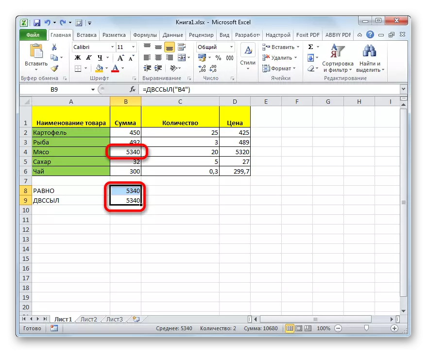
Consider what it means on the simplest example. In cells B8 and B9, respectively, placed recorded through the "=" formula and the function of the dwarf. Both formulas refer to the element B4 and output its contents on the sheet. Naturally this content is the same.

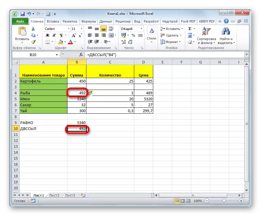
Add another empty element to the table. As you can see, the rows moved. In the formula using "equal", the value remains the same, as it refers to the final cell, even if its coordinates have changed, but the data from the operator by the operator has changed. This is due to the fact that it refers not to the leaf element, but on the coordinates. After adding a string, the address B4 contains another sheet element. Its content is now formula and displays on the sheet.

This operator is capable of displaying not only the number, but also the text, the result of the calculation of formulas and any other values ​​that are located in the selected sheet element. But in practice, this function is rarely used independently, and much more often is an integral part of complex formulas.

It should be noted that the operator is applicable for references to other sheets and even on the contents of other Excel books, but in this case they must be launched.

Now let's consider specific examples of the application of the operator.

Example 1: Single application of the operator

To begin with, consider the simplest example in which the Film Function protrudes independently so that you can understand the essence of her work.

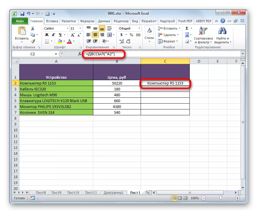
We have an arbitrary table. There is a task to display the first cell data of the first column in the first element of the individual column using the studied formula.

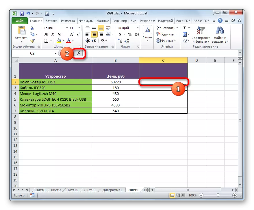
1. We highlight the first empty element of the column, where we plan to insert the formula. Click on the "Insert function" icon.



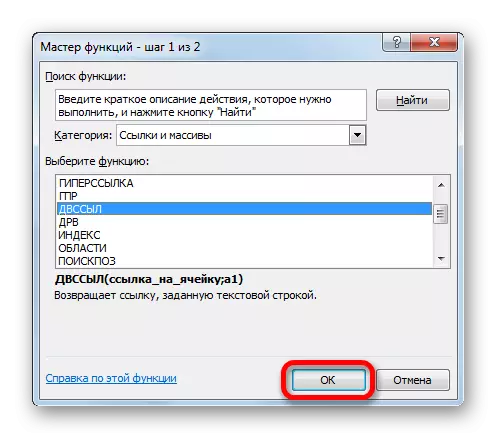
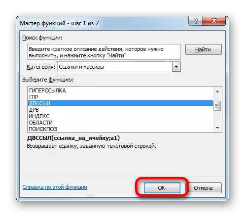
2. The functions wizard window starts running. We move to the category "Links and arrays". From the list, select the value "DVSSL". Click on the "OK" button.



3. The argument window of the specified operator is launched. In the "Link to the cell" field, you must specify the address of that element on the sheet, the contents of which we will display. Of course, it can be entered manually, but much more practical and it will be more convenient to do the following. Install the cursor in the field, then click the left mouse button on the appropriate element on the sheet. As you can see, immediately after that, its address appeared in the field. Then we allocate the link with quotes from both sides. As we remember, this is a feature of working with the argument of this formula.

   In the "A1" field, since we work in the usual type of coordinate, you can put the value of "truth", and you can leave it at all empty that we will do. These will be equivalent actions.

   After that, click on the "OK" button.



4. As we see, now the contents of the first cell of the first column of the table are displayed in the element of the sheet in which the formula is located.



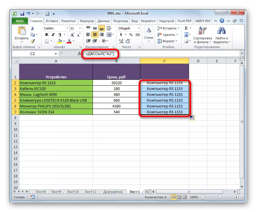
5. If we want to apply this function in the cells, which are located below, then in this case you will have to be administered to each element formula separately. If we try to copy it using a filling marker or another copying method, the same name will be displayed in all elements of the column. The fact is that, as we remember, the reference acts as an argument in text form (wrapped in quotes), which means that it cannot be relative.

Lesson: Wizard Functions in Excel Program

Example 2: Using an operator in a comprehensive formula

And now let's look at the example of a much more frequent use of the two operator, when it is an integral part of the complex formula.

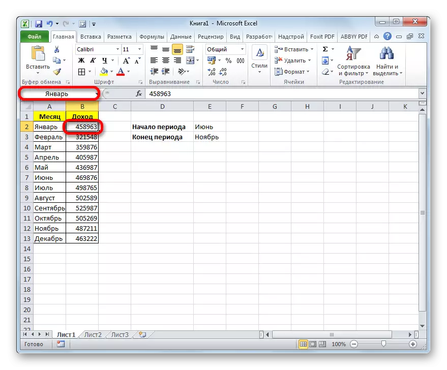
We have a monthly table of enterprise income. We need to calculate the amount of income for a certain period of time, for example Mart - May or June - November. Of course, for this, it is possible to use the formula for simple summation, but in this case, if necessary, counting the general result for each period, we will have to change this formula all the time. But when using the function, the dwarf can be changed by the summable range, simply specifying the corresponding month in individual cells. Let's try to use this option in practice first to calculate the amount for the period from March to May. This will use the formula with a combination of state operators and dash.

1. First of all, in individual elements on a sheet of the name of the months of the beginning and end of the period, for which the calculation will be calculated, respectively, "March" and "May".



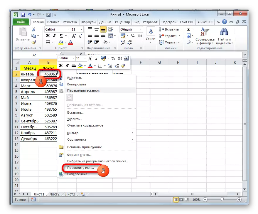
2. Now we assign the name to all cells in the "Income" column, which will be similar to the name of the corresponding month. That is, the first element in the "Income" column, which contains the size of the revenue, should be called "January", the second - "February", etc.

   So, to assign the name to the first element of the column, select it and press the right mouse button. The context menu opens. Select the item "Assign Name ...".



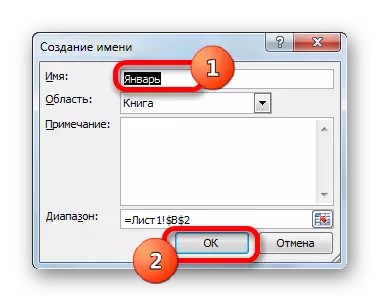
3. The name creation window is launched. In the "Name" field fit the name "January". No more changes in the window do not need to be done, although just in case you can check that the coordinates in the "range" field correspond to the cell's address containing revenue size in January. After that, click on the "OK" button.



4. As you can see, now, when you allocate this item in the name window, it is not displayed for its address, and then the name we gave her. A similar operation is done with all other elements of the "income" column, giving them consistently named "February", "March", "April", etc. until December inclusive.



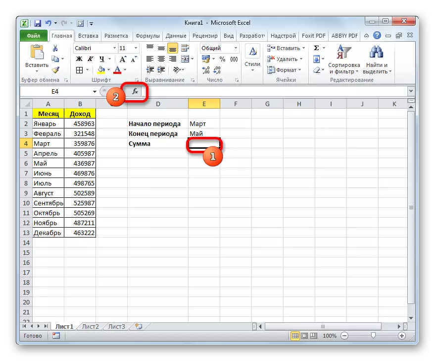
5. Select the cell into which the sum of the values ​​of the specified interval will be displayed and allocate it. Then click on the "Insert function" icon. It is placed on the left of the line of formulas and to the right of the field where the name of the cells is displayed.



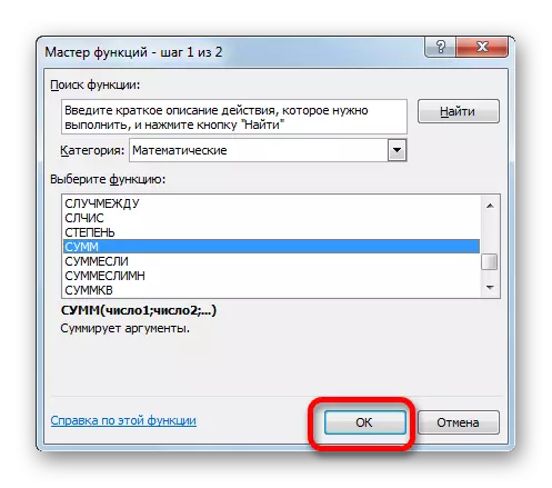
6. In the activated window, the masters of functions move to the category "Mathematical". There choose the name "sums". Click on the "OK" button.



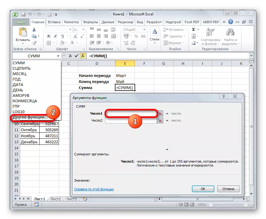
7. Following the execution of this action, the Operator arguments window is launched, the only task of which is the summation of the specified values. The syntax of this function is very simple:

   = Sums (number1; number2; ...)

   In general, the number of arguments can reach the values ​​of 255. But all these arguments are homogeneous. They are the number or coordinates of the cell in which this number is contained. They can also perform in the form of a built-in formula that calculates the desired number or indicates the address of the leaf element where it is placed. It is in this quality of the built-in function and our operator will be used in this case.

   Install the cursor in the "Number1" field. Then click on the icon in the form of an inverted triangle to the right of the range of the ranges. The list of recent functions used is disclosed. If there is a "DVSSL" name among them, then immediately click on it to go to the argument window of this function. But it may well be that in this list you will not find it. In this case, you need to click on the name "Other functions ..." at the bottom of the list.



8. Launched already familiar to us window wizard functions. We move to the section "Links and arrays" and choose the name of the operator DVSSL. After that, you click on the "OK" button at the bottom of the window.



9. The window of the operator's arguments of the operator is launched. In the "Link to the cell" field, specify the address of the leaf element, which contains the name of the initial month of the range intended for calculating the amount. Please note that in this case you do not need to take a link in quotes, since in this case there will be no cell coordinates, but its contents, which already has a text format (the word "March"). The "A1" field is left blank, since we use the standard coordinate designation type.

   After the address is displayed in the field, do not rush to the "OK" button, as this is a nested function, and the actions with it differ from the usual algorithm. Click on the name "sums" in the line of formulas.



10. After that, we return to the arguments of the sums. As you can see, the "Number1" field has already disappeared the operator twisted with its contents. Install the cursor in the same field immediately after the last symbol in the record. Put the sign of the colon (:). This symbol means the address sign of the cell range. Next, without removing the cursor from the field, again click on the icon as a triangle for selecting functions. This time in the list of recently used operators, the name "DVSSL" should be considered accurate, as we recently used this feature. Click by name.



11. The arguments of the operator's arguments of the operator opens again. We enter the "Link to the cell" field the address of the element on the sheet where the name of the month is located, which completes the estimated period. Again the coordinates must be inscribed without quotes. The field "A1" leave empty again. After that, click on the "OK" button.



12. As you can see, after these actions, the program makes a calculation and gives the result of the addition of the enterprise's income for the specified period (March - May) into the pre-dedicated element of the sheet in which the formula itself is located.



13. If we change in cells, where the names of the beginnings and the end of the estimated period are inscribed, for others, for example, on June and November, and the result will change accordingly. The amount of income for the specified period of time will be folded.

Lesson: How to calculate the amount in Excel

As we can see, despite the fact that the FVS function cannot be called one of the most popular users, however, it helps to solve the tasks of various difficulties in Excel is much easier than it could be done with other tools. Most of all this operator is useful as part of complex formulas in which it is an integral part of the expression. But still it should be noted that all the possibilities of the operator dock are quite severe for understanding. This is just explaining the lowest popularity of this useful function from users.