Cell color depending on the value in Excel

When working with tables, the priority value has the values ​​displayed in it. But an important component is also its design. Some users consider it a secondary factor and do not pay special attention to him. And in vain, because a beautifully decorated table is an important condition for better perception and understanding by users. The visualization of data is particularly played in this. For example, using visualization tools, you can paint the table cells depending on their contents. Let's find out how it can be done in the Excel program.

The procedure for changing the color of the cells depending on the contents

Of course, it is always nice to have a well-designed table, in which cells depending on the contents are painted in different colors. But this feature is particularly relevant for large tables containing a significant data array. In this case, the fill with the color of the cells will greatly facilitate users orientation in this huge amount of information, as it can be said will be already structured.

Leaf elements can be attempting to manually paint, but again, if the table is large, it will take a considerable amount of time. In addition, in such an array of data, the human factor can play a role and errors will be allowed. Not to mention the table can be dynamic and the data in it periodically change, and massively. In this case, manually change the color in general it becomes unreal.

But the output exists. For cells that contain dynamic (changing) values ​​applied conditional formatting, and for statistical data you can use the "Find and Replace" tool.

Method 1: Conditional formatting

Using conditional formatting, you can specify certain boundaries of the values ​​in which the cells will be painted in one color. Staining will be carried out automatically. In case the cell value, due to the change, will be out of the boundary, it will automatically repaint this leaf element.

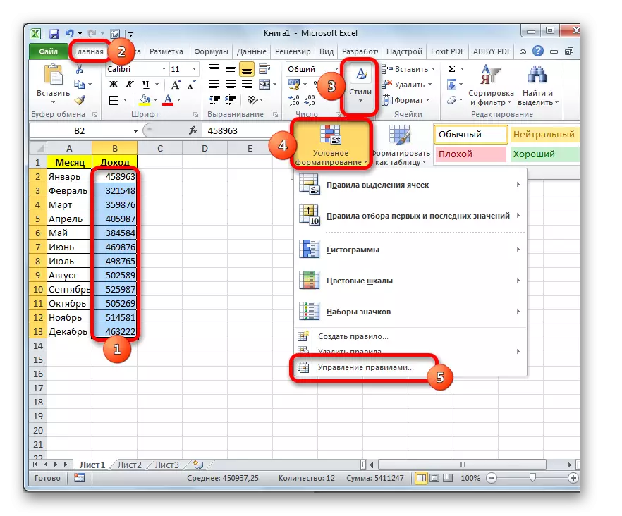
Let's see how this method works on a specific example. We have a table of income of the enterprise, in which these data is afraid. We need to highlight with different colors those elements in which the amount of income is less than 400,000 rubles, from 400,000 to 500,000 rubles and exceeds 500,000 rubles.

1. We highlight the column in which information on the income of the enterprise is located. Then we move to the "Home" tab. Click on the "Conditional Formatting" button, which is located on the tape in the "Styles" tool block. In the list that opens, select the rules management item.



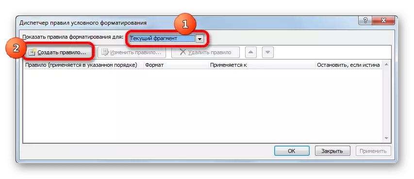
2. The conventional formatting rules are launched. The "Show Formatting Rule for" field must be set to the "Current Fragment" value. By default, it is precisely it should be listed there, but just in case, check and in case of inconsistency, change the settings according to the above recommendations. After that, click on the "Create Rule ..." button.



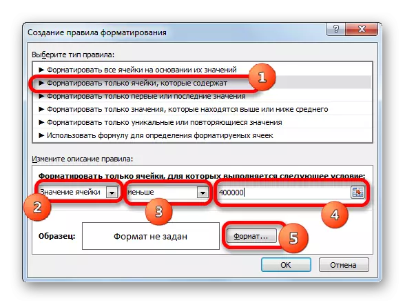
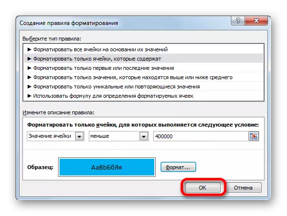
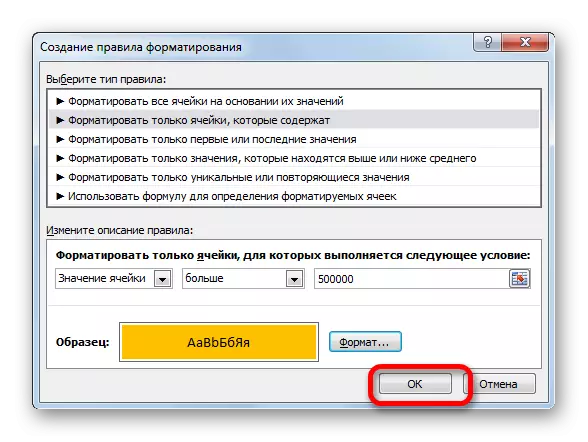
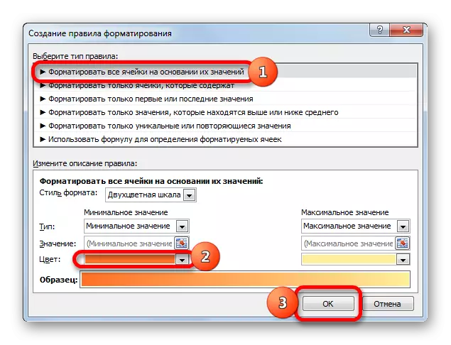
3. The formatting rule creation window opens. In the list of types of rules, select the position "Format only cells that contain". In the description block, the Rules in the first field, the switch must stand in the "Value" position. In the second field, we set the switch to the "less" position. In the third field, specify the value, the elements of the sheet containing the amount of which will be painted in a certain color. In our case, this value will be 400,000. After that, we click on the "Format ..." button.



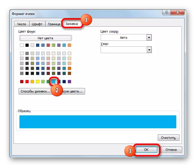
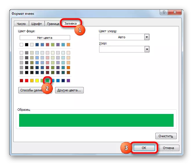
4. Cell format window opens. Move into the "Fill" tab. Choose the color of the fill that we wish, to stand out cells containing a value of less than 400,000. After that, we click on the "OK" button at the bottom of the window.



5. We return to the creation window of the formatting rule and there, too, click on the "OK" button.



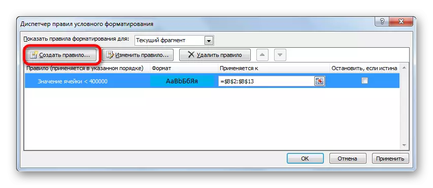
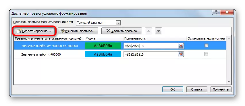
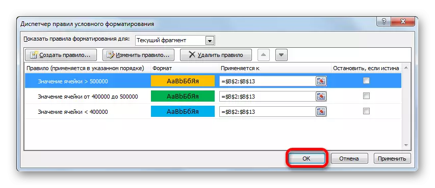
6. After this action, we will again be redirected to the Conditional Formatting Rules Manager. As you can see, one rule has already been added, but we have to add two more. Therefore, we press the "Create Rule ..." button again.



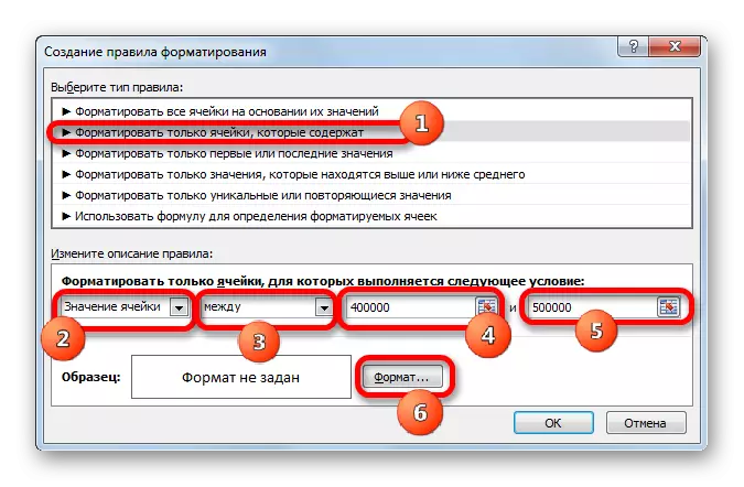
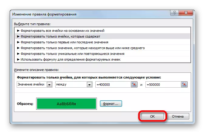
7. And again we get into the creation window. Move into the section "Format only cells that contain". In the first field of this section, we leave the "Cell value" parameter, and in the second set the switch to the "Between" position. In the third field, you need to specify the initial value of the range in which the elements of the sheet will be formatted. In our case, this is the number 400000. In the fourth, specify the final value of this range. It will be 500,000. After that, click on the "Format ..." button.



8. In the formatting window, we move back to the "Fill" tab, but this time already choose another color, then click on the "OK" button.



9. After returning to the creation window, I also click on the "OK" button.



10. As we see, two rules have already been created in the rules manager. Thus, it remains to create a third. Click on the "Create Rule" button.



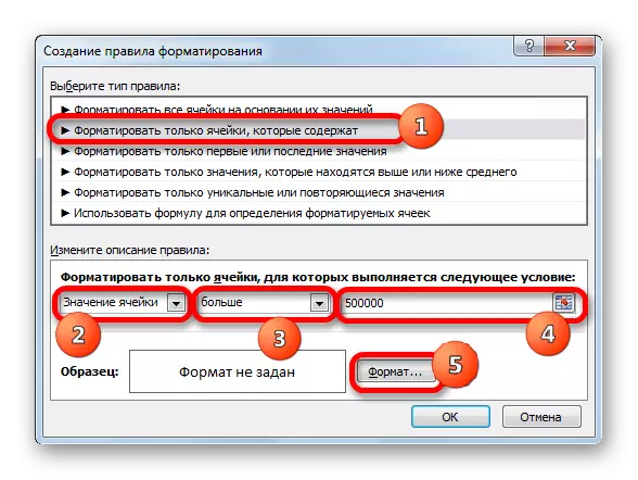
11. In the Creation of the Rules window, again move to the section "Format only cells that contain". In the first field, we leave the option "Cell value". In the second field, install the switch to the "More" police. In the third field, drive the number 500000. Then, as in the previous cases, we click on the "Format ..." button.



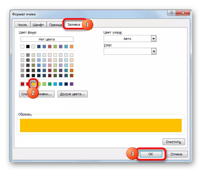
12. In the "Format of Cells", again move to the "Fill" tab. This time we choose a color that differs from the two previous cases. Perform a click on the "OK" button.



13. In the Rules' Creation window, repeat pressing the "OK" button.



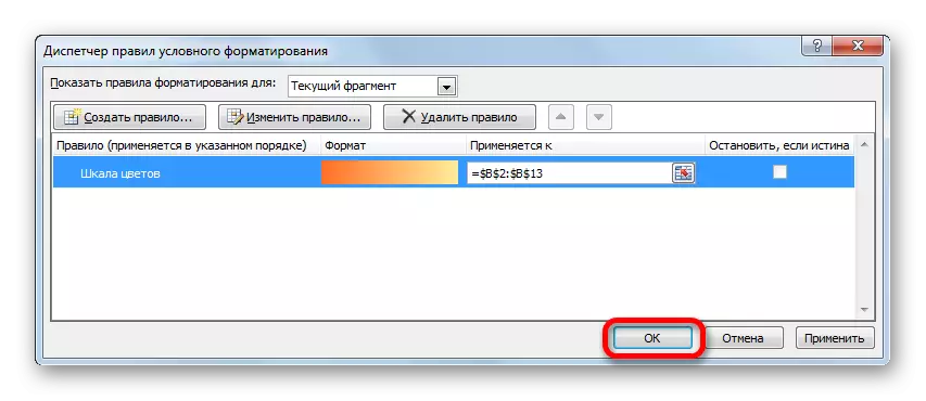
14. The rules dispatcher opens. As you can see, all three rules are created, so we press the "OK" button.



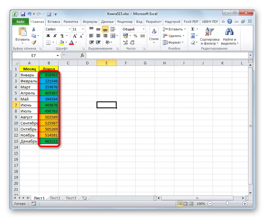
15. Now the elements of the table are painted according to the specified conditions and borders in the conditional formatting settings.



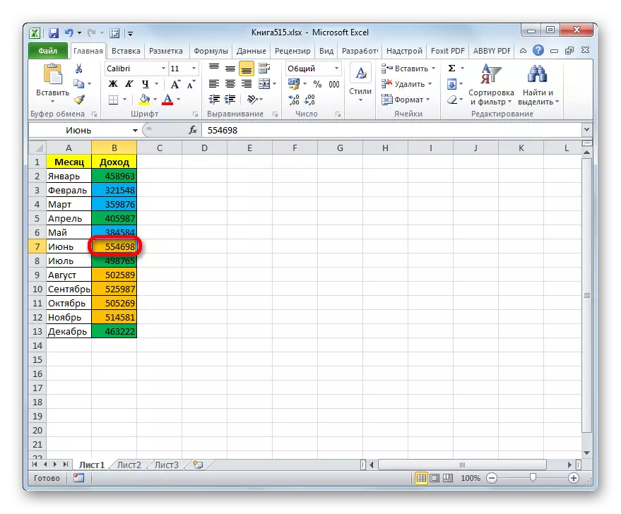
16. If we change the contents in one of the cells, leaving the boundaries of one of the specified rules, then this element of the sheet will automatically change color.

In addition, it is possible to use conditional formatting somewhat differently for the color of the sheet elements in color.

1. For this, after the rules manager, we go to the formatting window, we stay in the "Format all cells based on their values" section. In the "Color" field, you can choose that color, the shades of which will be poured the elements of the sheet. Then you should click on the "OK" button.



2. In the rules manager, too, press the "OK" button.



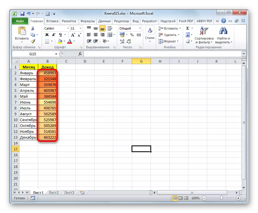
3. As you can see, after this cell in the column is painted with various shades of the same color. The value that the sheet element contains is larger, the lower is lighter than less - the darker.

Lesson: Conditional formatting in Excele

Method 2: Using the "Find and Allocate" tool

If there are static data in the table, which are not planned to be changed over time, you can use the tool to change the color of the cells by their content called "Find and Allocate". The specified tool will allow you to find the specified values ​​and change the color in these cells to the user you need. But it should be noted that when changing the contents in the sheet elements, the color will not automatically change, but remains the same. In order to change the color to the relevant, you will have to repeat the procedure again. Therefore, this method is not optimal for tables with dynamic content.

Let's see how it works on a specific example, for which we take the same table of income of the enterprise.

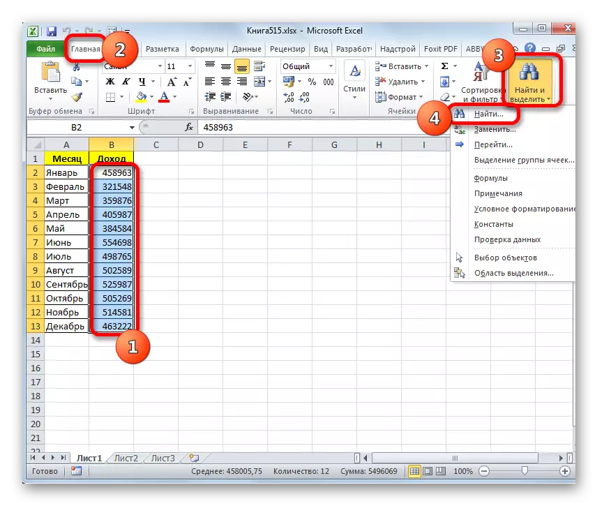
1. We highlight a column with data that should be formatted by color. Then go to the "Home" tab and click on the "Find and Select" button, which is located on the tape in the Editing toolbar. In the list that opens, click on "Find".



2. The "Find and Replace" window starts in the "Find" tab. First of all, we will find values ​​up to 400,000 rubles. Since we have no cell, where there would be less than 300,000 rubles, then, in fact, we need to highlight all the elements in which numbers are in the range from 300,000 to 400,000. Unfortunately, directly indicate this range, as in the case Applications of conditional formatting, in this method it is impossible.

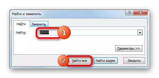
   But there is a possibility to do somewhat differently that we will give the same result. You can set the following template "3 ????? in the search bar. A question mark means any character. Thus, the program will look for all six-digit numbers that begin with the numbers "3". That is, the search for search will fall in the range of 300,000 - 400,000, which we are required. If the table had numbers less than 300,000 or less than 200,000, then for each range in a hundred thousand, the search would have to be done separately.

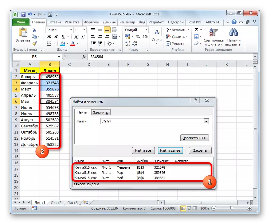
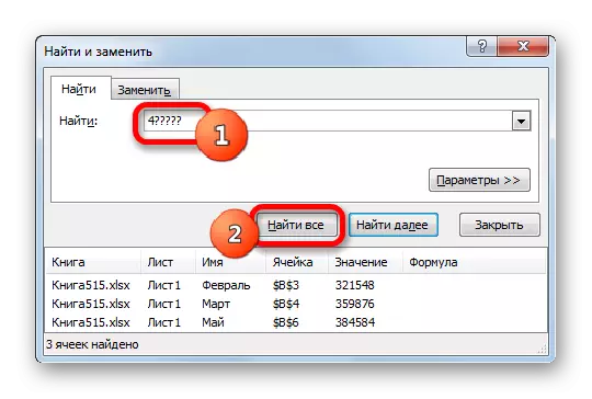
   We introduce the expression "3 ?????" In the "Find" and click on the "Find All" button.



3. After that, in the lower part of the window, the results of search results are open. Click on the left mouse button on any of them. Then you type the Ctrl + A key combination. After that, all the results of the search for issuing are allocated and the elements in the column are distinguished at the same time, to which these results refer.



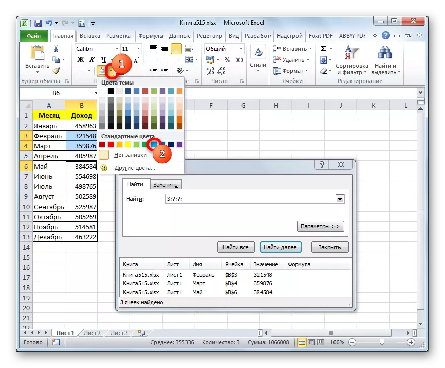
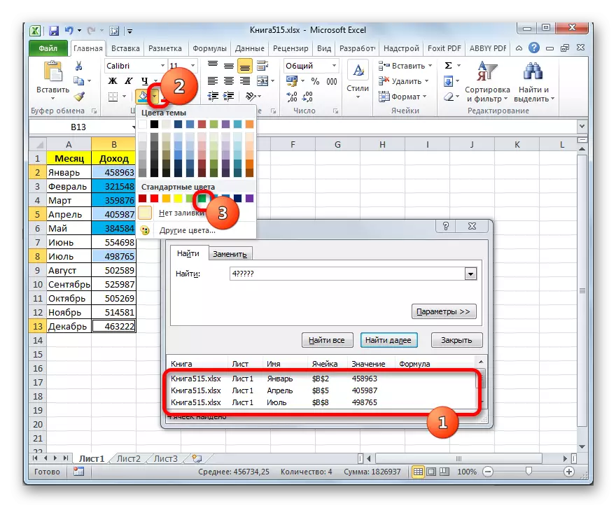
4. After the elements in the column are highlighted, do not rush to close the "Find and Replace" window. Being in the "Home" tab in which we have moved earlier, go to the tape to the font tool block. Click on the triangle to the right of the "Fill color" button. There is a choice of different colors of the fill. Choose the color that we want to apply to the elements of a sheet containing values ​​less than 400,000 rubles.



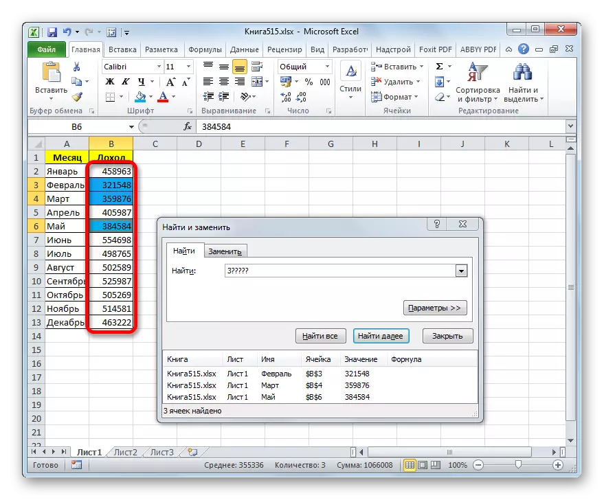
5. As you can see, all cells of the column in which there are less than 400,000 rubles are highlighted, highlighted in the selected color.



6. Now we need to paint the elements in which the quantities are located in the range from 400,000 to 500,000 rubles. This range includes numbers that match the "4 ??????" template. We drive it into the search field and click on the "Find all" button, after selecting the column you need.



7. Similarly, with the previous time in the search for issuance, we allocate the entire result obtained by pressing the Ctrl + A hot key combination. After that, we move to the fill color selection icon. Click on it and click on the icon of the shade you need, which will be painted the elements of the sheet, where the values ​​are in the range from 400,000 to 500,000.



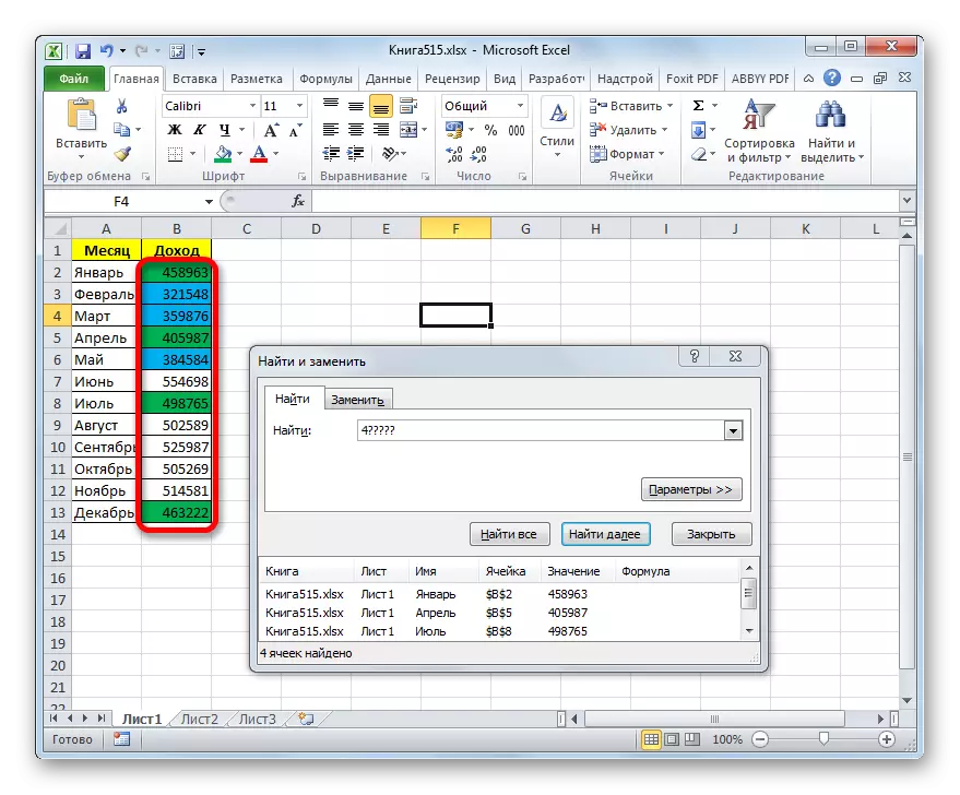
8. As you can see, after this action, all the elements of the table with data in the range from 400,000 to 500,000 are highlighted in the selected color.



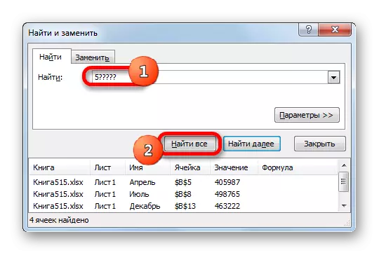
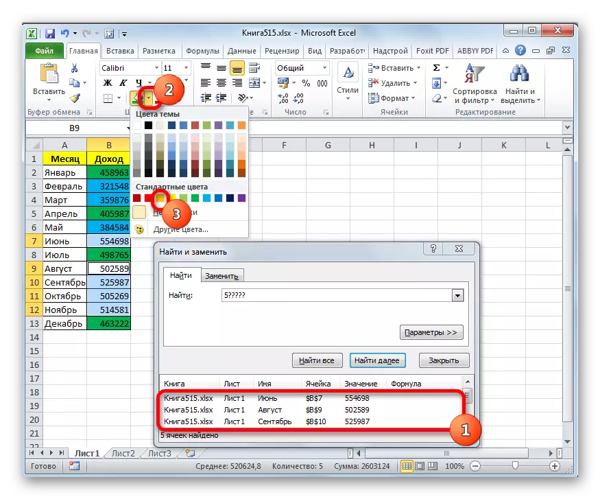
9. Now we have to highlight the last interval values ​​- more than 500,000. Here we are too lucky, since all the numbers more than 500,000 are in the range from 500,000 to 600,000. Therefore, in the search field we introduce the expression "5 ?????" And click on the "Find all" button. If there were values ​​exceeding 600,000, then we would need to additionally search for expression "6 ?????" etc.



10. Again, allocate search results using Ctrl + A combination. Next, using the tape button, select a new color to fill the interval exceeding 500000 for the same analogy as we did before.



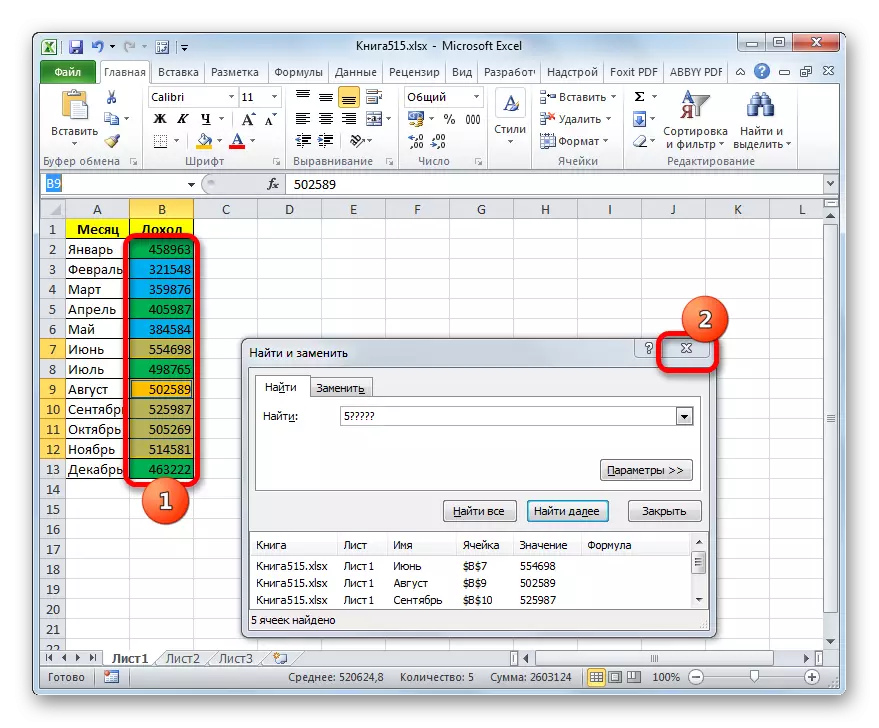
11. As you can see, after this action, all elements of the column will be painted, according to the numerical value, which is placed in them. Now you can close the search box by pressing the standard closing button in the upper right corner of the window, since our task can be considered solved.



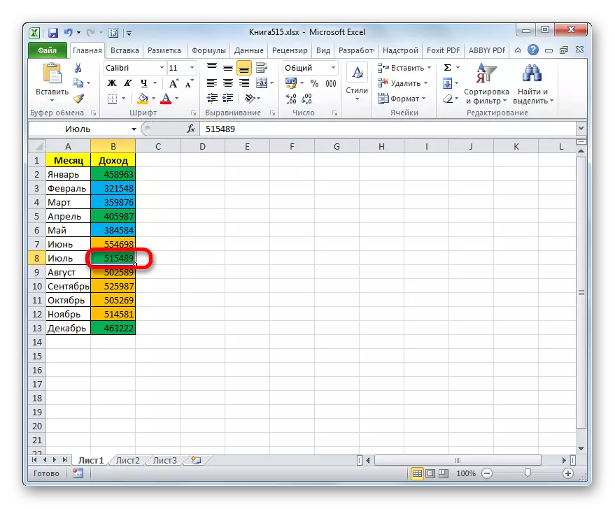
12. But if we replace the number to another, which goes beyond the borders that are installed for a specific color, the color will not change, as it was in the previous way. This suggests that this option will work reliably only in those tables in which the data does not change.

Lesson: How to make a search in exale

As you can see, there are two ways to paint the cells depending on the numerical values ​​that are in them: with the help of conditional formatting and using the "Find and Replace" tool. The first method is more progressive, as it allows you to more clearly specify the conditions for which the elements of the sheet will be distinguished. In addition, when conditional formatting, the element color is automatically changing, in case of changing the contents in it, which cannot be done. However, the fill of the cells, depending on the value by applying the "Find and Replace" tool, is also quite used, but only in static tables.