Absolute Addressing in Excel: 2 proven method

As you know, there are two types of addressing in Excel tables: relative and absolute. In the first case, the reference varies in the direction of copying to the relative shift value, and in the second, it is fixed and when copying remains unchanged. But by default, all addresses in Excel are absolute. At the same time, quite often there is a need to use an absolute (fixed) addressing. Let's find out what methods this can be done.

Application of absolute addressing

Absolute addressing we may need, for example, in the case when we copy the formula, one part of which consists of a variable displayed in a number of numbers, and the second has a constant value. That is, this number plays the role of the constant coefficient, with which a certain operation must be carried out (multiplication, division, etc.) of the number of variables.

In Excel, there are two ways to set a fixed addressing: by forming an absolute link and with the help of the FVS function. Let's consider each of these ways in detail.

Method 1: Absolute Link

Of course, the most famous and frequently applied way to create an absolute addressing is the use of absolute links. Absolute references have the difference not only functional, but also syntax. The relative address has such a syntax:

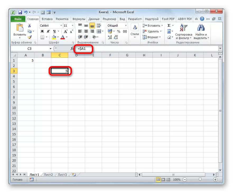
= A1.

At the fixed address before the coordinate value sets the dollar sign:

= $ A $ 1

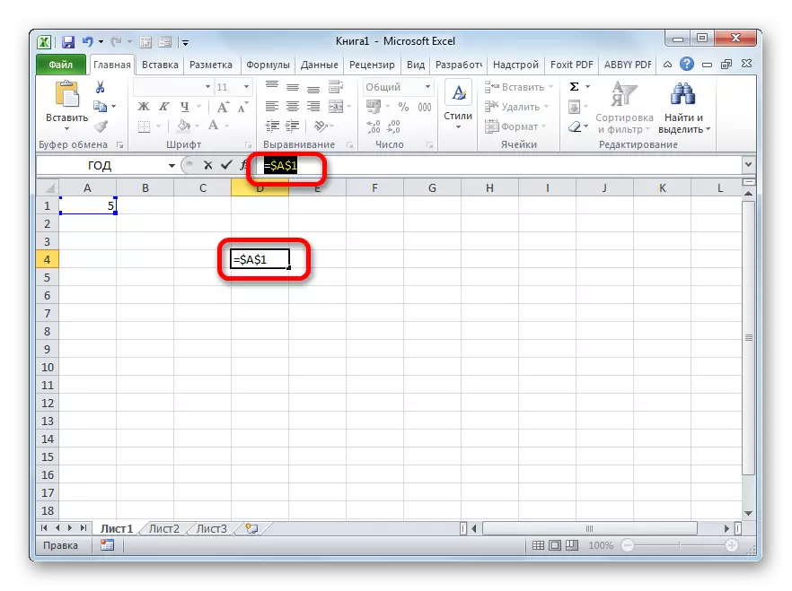
Dollar sign can be entered manually. To do this, you need to install the cursor before the first value of the coordinates of the address (horizontally) located in the cell or in the formula row. Next, in the English-speaking keyboard layout, click on the "4" key in the upper case (with the "SHIFT" key). It is there that the dollar symbol is located. Then you need to do the same procedure with the coordinates of the vertical.

There is a faster way. You need to set the cursor to the cell in which the address is located and click on the F4 function key. After that, the dollar sign will instantly appear simultaneously before coordinates horizontally and vertically this address.

Now let's consider how the absolute addressing is used in practice by using absolute links.

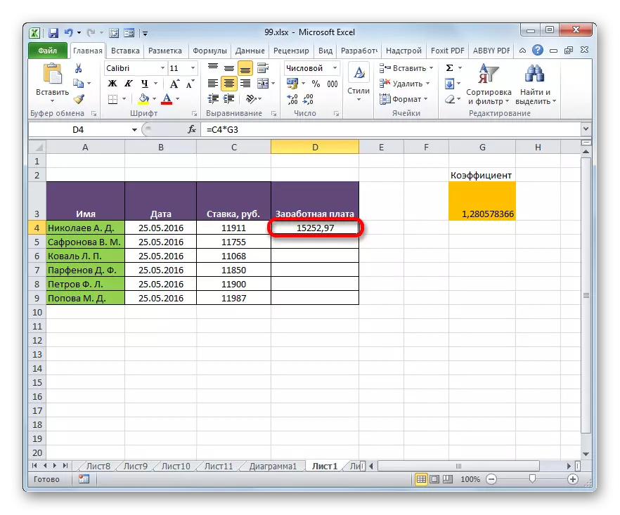
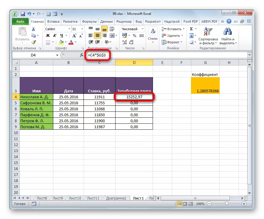
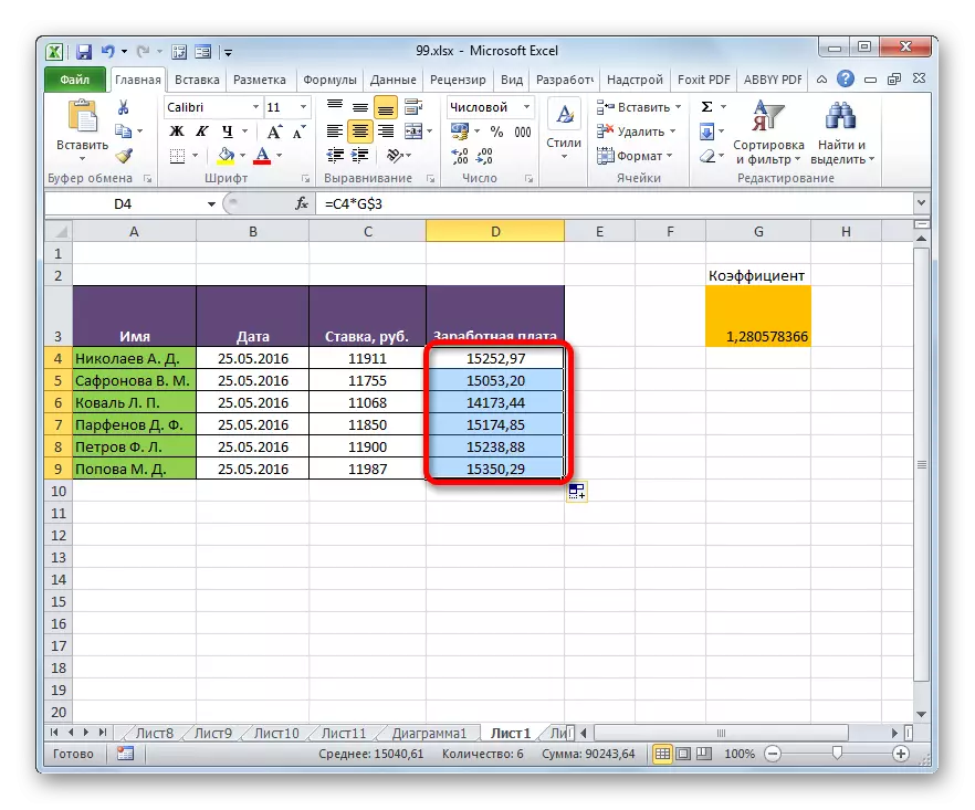
Take the table in which the salary of workers is calculated. The calculation is made by multiplying the magnitude of their personal salary to the fixed coefficient, which is the same for all employees. The coefficient itself is located in a separate leaf cell. We are faced with the task of calculating the wages of all workers as fast as possible.

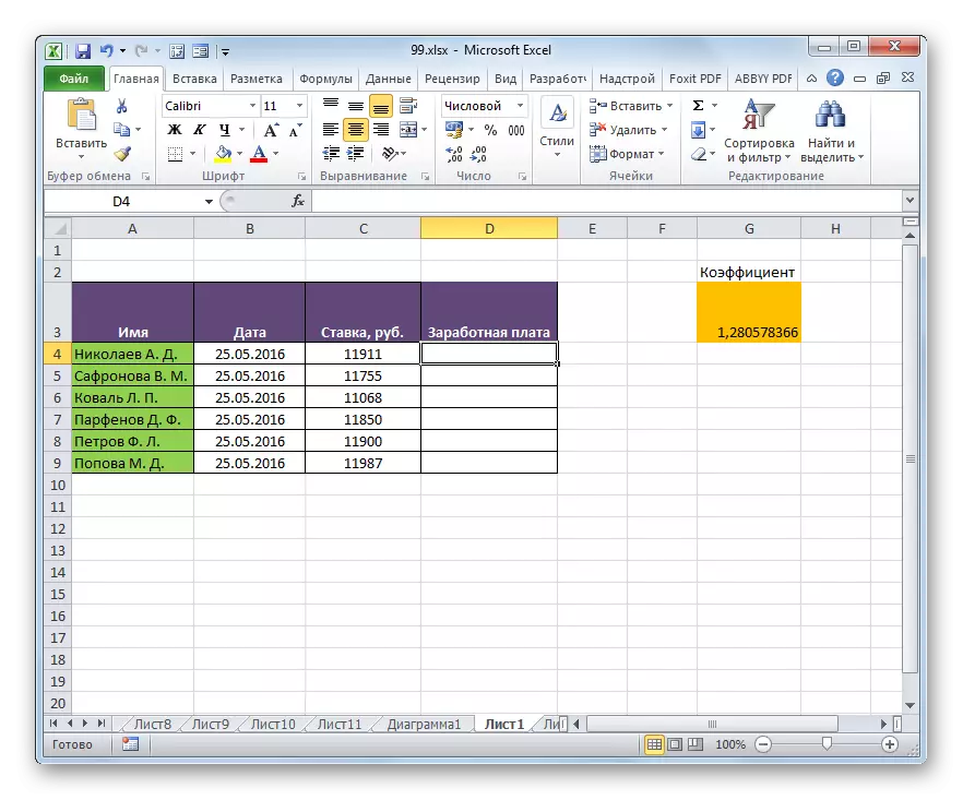
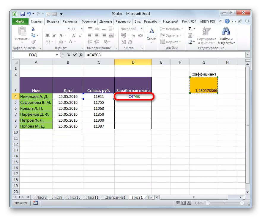
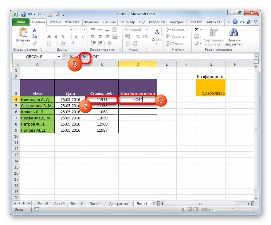
1. So, in the first cell of the wage column, we introduce the formula for multiplying the rate of the relevant employee to the coefficient. In our case, this formula has this kind:

   = C4 * G3



2. To calculate the finished result, click the Enter key on the keyboard. The result is displayed in a cell containing the formula.



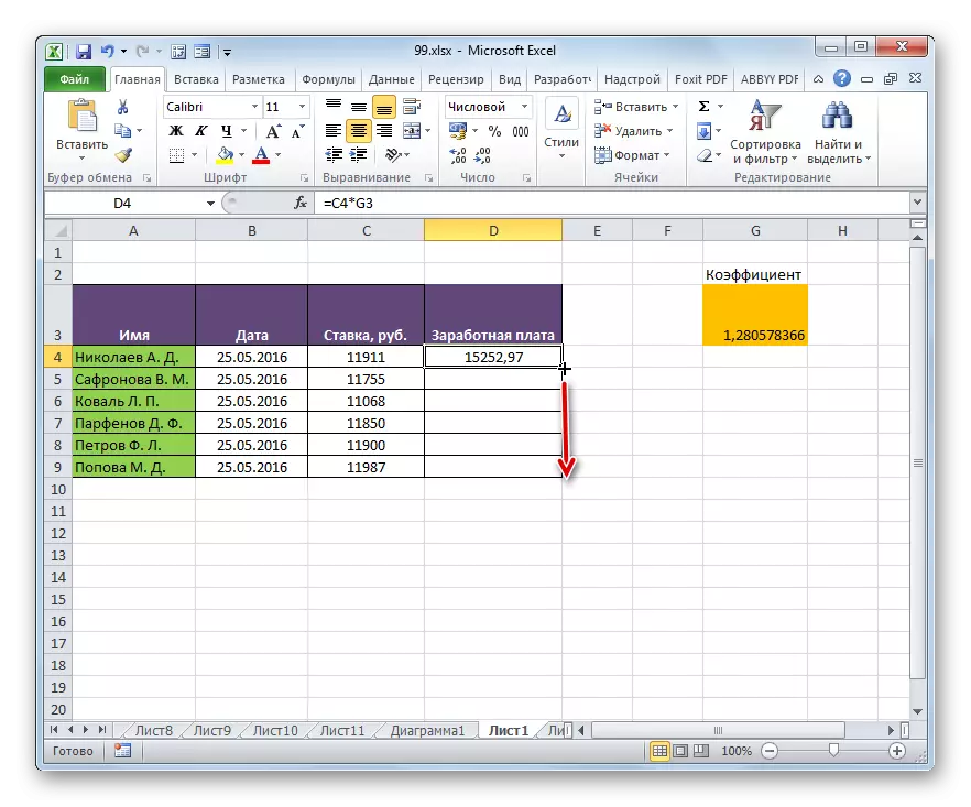
3. We calculated the value of the salary for the first employee. Now we need to do it for all other lines. Of course, the operation can be written in each cell "Wages" column manually, introducing a similar formula with an amendment to the offset, but we have a task as quickly as possible to calculate, and the hand-made input will take a large amount of time. And why spend efforts on manual input, if the formula is simply copied to other cells?

   To copy the formula, we apply such a tool as a filling marker. We become a cursor to the lower right corner of the cell, where it is contained. At the same time, the cursor itself must transform into this very marker of filling in the form of a cross. Push the left mouse button and pull the cursor down to the end of the table.



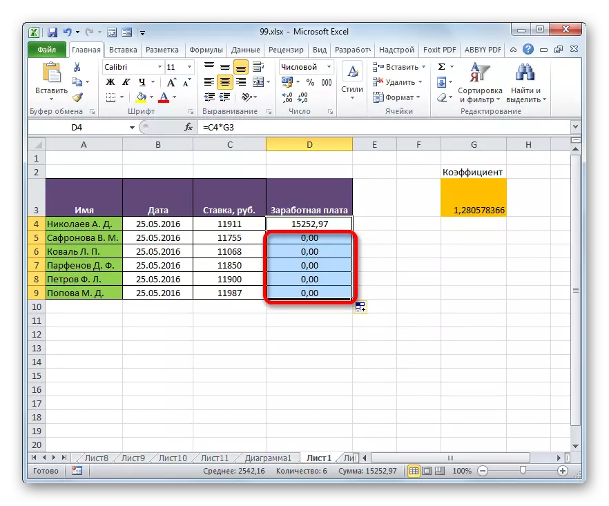
4. But, as we see, instead of the correct calculation of wages for other employees, we got some zeros.



5. We look at what the reason for this result. To do this, we highlight the second cell in the Salary column. The formula string displays the corresponding expression on this cell. As you can see, the first factor (C5) corresponds to the rate of that employee whose salary we expect. Coordinate displacement compared to the previous cell due to the properties of relativity. However, in specifically this case, this is necessary for us. Thanks to this first multiplier, the rate of the employee we need was. But the coordinate displacement occurred with the second factor. And now its address refers not to the coefficient (1.28), but on the empty cell below.

   

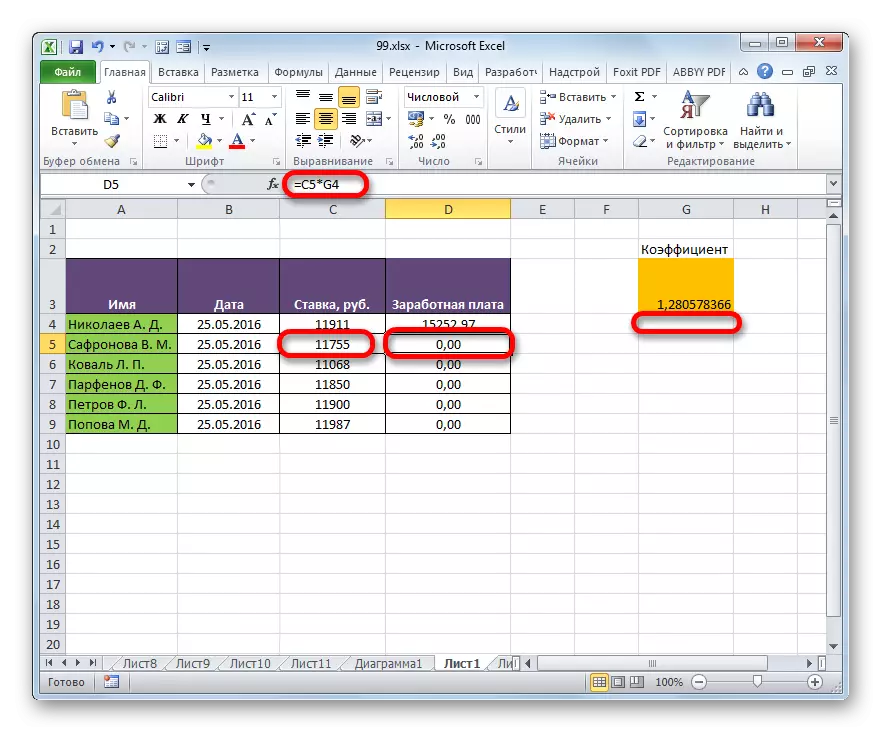
   This is exactly the reason for calculating the salary for subsequent employees from the list turned out to be incorrect.

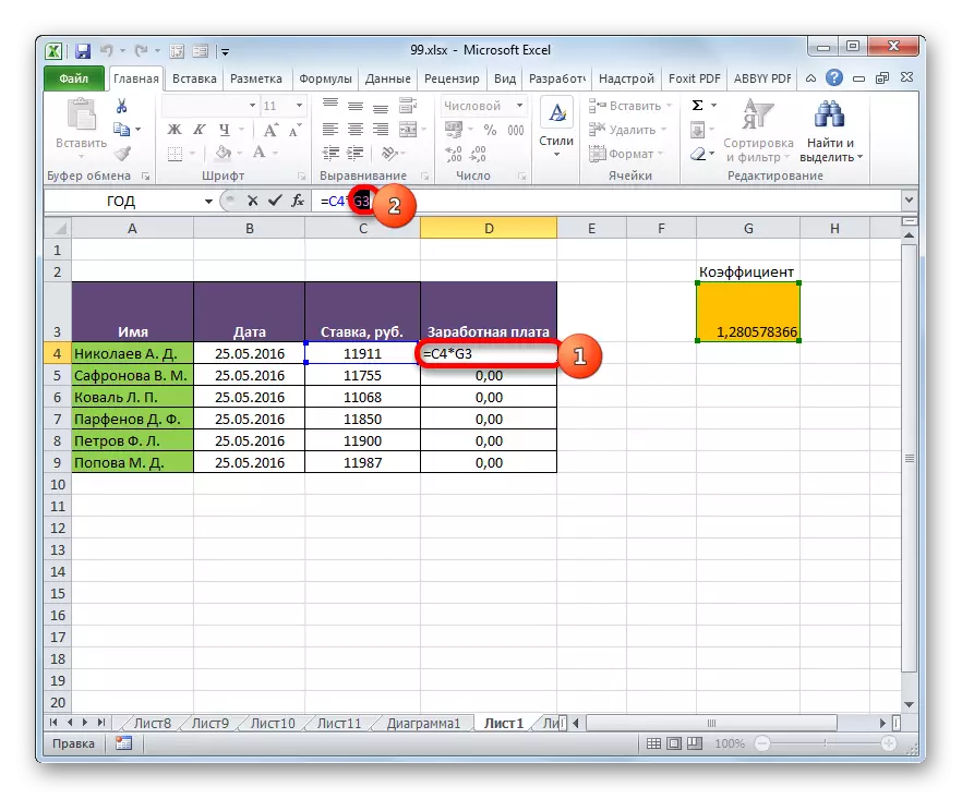
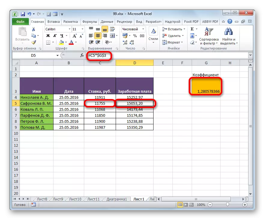
6. To correct the situation, we need to change the addressing of the second multiplier with a relative to fixed. To do this, we return to the first cell of the "Salary" column, highlighting it. Next, we move to the string of formulas where the expression we need is displayed. We highlight the cursor the second factor (G3) and press the soft key on the keyboard.



7. As we see, a dollar sign appeared near the coordinates of the second factor, and this, as we remember, is the attribute of absolute addressing. To display the result on the screen we click on the ENTER key.



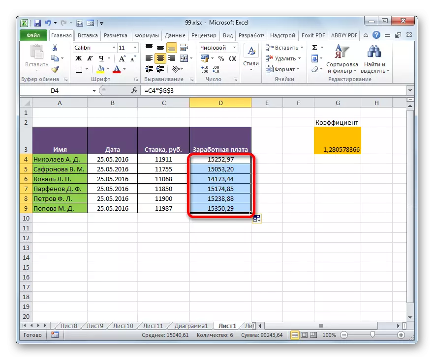
8. Now, as before, we call the fill marker by installing the cursor to the lower right angle of the first element of the wage column. Push the left mouse button and pull it down.



9. As we see, in this case the calculation was carried out correctly and the amount of wages for all employees of the enterprise is calculated correctly.



10. Check how the formula was copied. To do this, we allocate the second element of the wage column. We look at the expression located in the formula row. As we see, the coordinates of the first factor (C5), which is still relative, moved compared to the previous cell to one point down vertically. But the second factor ($ G $ 3), the addressing in which we made fixed remained unchanged.

Excel also uses the so-called mixed addressing. In this case, either a column or a string is recorded in the element address. This is achieved in such a way that the dollar sign is placed only before one of the address coordinates. Here is an example of a typical mixed link:

= A $ 1

This address is also considered mixed:

= $ A1

That is, the absolute addressing in a mixed link is used only for one of the coordinate values ​​of two.

Let's see how such a mixed link can be applied to practice on the example of the same salary table of employees of the enterprise.

1. As we can see, earlier we did so that all coordinates of the second multiplier have absolute addressing. But let's figure it out if both values ​​must be fixed in this case? As we see, when copying, a vertical shift occurs, and the horizontal coordinates remain unchanged. Therefore, it is quite possible to apply the absolute addressing only to the coordinates of the line, and the column coordinates should be left as they are the default - relative.

   We allocate the first element of the wage column and in the formula string, we perform the above manipulation. We get the formula for the following type:

   = C4 * G $ 3

   As we can see, a fixed addressing in the second multiplier applies only in relation to the coordinates of the string. To display the result in the cell click the ENTER button.



2. After that, through the filling marker, copy this formula on the range of cells, which is located below. As you can see, the salary calculation for all employees is performed correctly.



3. We look at how the copied formula is displayed in the second cell of the column over which we performed manipulation. As can be observed in the formula row, after the selection of this element of the sheet, despite the fact that the absolute addressing of the second factor had only row coordinates, the coordinates of the column coordinate did not occur. This is due to the fact that we performed copying not horizontally, but vertically. If we were copying horizontally, then in a similar case, on the contrary, it would have to make a fixed addressing of column coordinates, and for the lines this procedure would be optional.

Lesson: Absolute and Relative Links in Excel

Method 2: Function Two

In the second way to organize an absolute addressing in the Excel table is the use of the operator DVSL. This feature refers to a group of built-in operators "Links and arrays". Its task is to form a reference to the specified cell with the output of the result in that element of the sheet in which the operator itself is. At the same time, the link is attached to the coordinates even stronger than when using the dollar sign. Therefore, it is sometimes taken to call references using Dultnsyl "Superable". This operator has the following syntax:

= Dwarf (link_namechair; [A1])

The function has two arguments, the first of which has a mandatory status, and the second is not.

The argument "Link to the cell" is a reference to an Excel sheet element in text form. That is, this is a regular link, but prisoner in quotes. This is exactly what allows you to ensure the properties of absolute addressing.

The argument "A1" is optional and used in rare cases. Its application is necessary only when the user selects an alternative addressing option, and not the usual use of coordinates by type "A1" (the columns have an alphabet designation, and the rows are digital). The alternative implies the use of the "R1C1" style, in which columns, like strings, are indicated by numbers. You can switch to this operation mode through the Excel parameters window. Then, using the operator DVSSL, as the argument "A1" should be specified the value "Lie". If you are working in the usual reference display mode, like most other users, then as an argument "A1" you can specify the value "Truth". However, this value is meant by default, so much easier in general in this case, the argument "A1" does not specify.

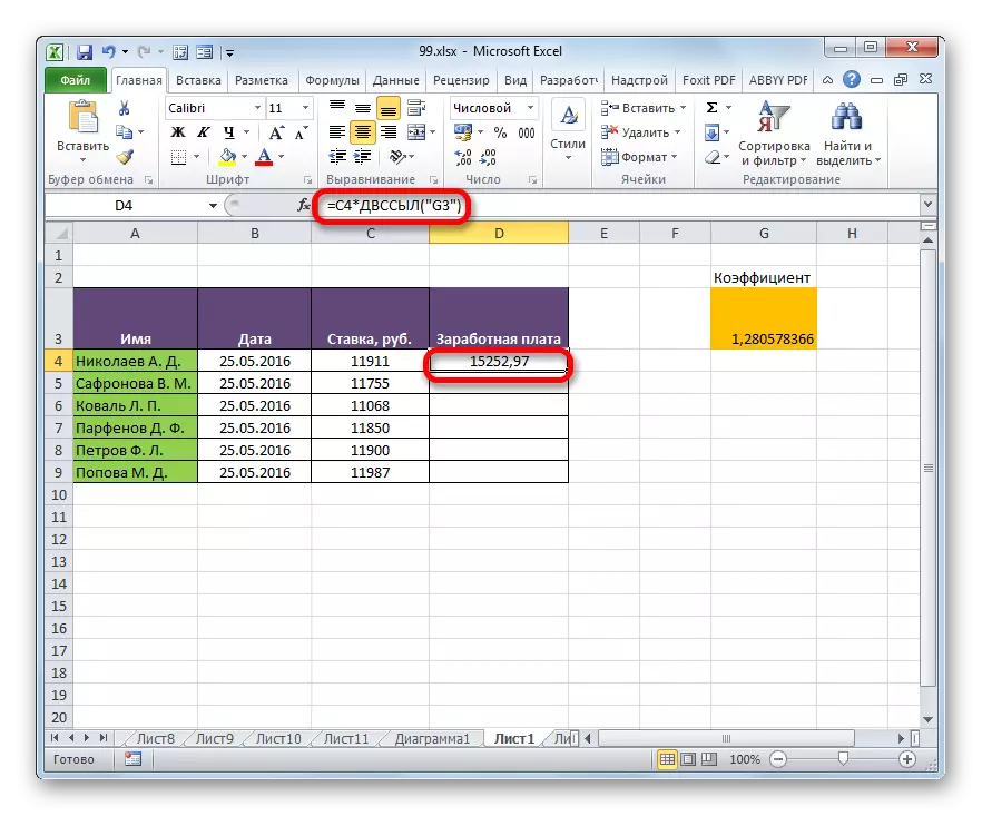
Let's take a look at how the absolute addressing will work, organized by the function of the DVRSL, on the example of our salary table.

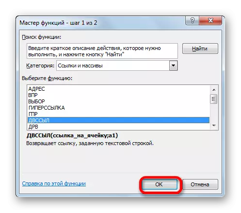
1. We produce the selection of the first element of the wage column. We put the sign "=". As remember, the first factor in the specified calculation formula must be submitted by the relative address. Therefore, just click on the cell containing the corresponding value of the salary (C4). Following how its address is displayed in the element to display the result, click on the "Multiply" button (*) on the keyboard. Then we need to go to the use of the operator DVSSL. Perform a click on the "Insert function" icon.



2. In the operating window of the Master of Functions, go to the category "Links and arrays". Among the named list of titles, we allocate the name "DVSSL". Then click on the "OK" button.



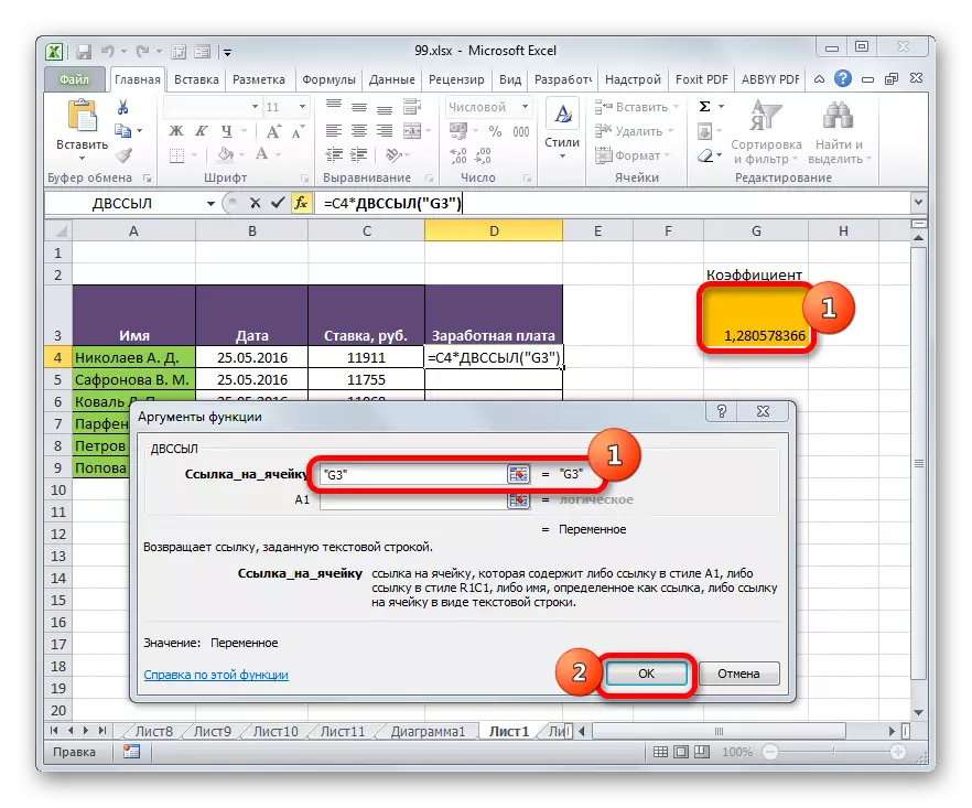
3. Activation of the arguments of the operator's arguments of DVSSL is made. It consists of two fields that correspond to the arguments of this function.

   We put the cursor in the Link to the Cell. Just click on that element of the sheet, in which the coefficient is located to calculate the salary (G3). The address will immediately appear in the Argument window field. If we were dealing with a conventional function, then on this addresses could be considered completed, but we use the FVS function. As we remember, the addresses in it should have the type of text. Therefore, turn around the coordinates that are located in the window field, quotes.

   Since we work in the standard coordinate display mode, then the field "A1" leave empty. Click on the "OK" button.



4. The application performs a calculation and outputs the result in the sheet element containing the formula.



5. Now we make copying this formula into all other cells of the wage column through the filling marker, as we did before. As you can see, all the results were calculated right.



6. Let's see how the formula is displayed in one of the cells, where it was copied. We highlight the second element of the column and look at the formula string. As you can see, the first factor, which is a relative reference, has changed its coordinates. At the same time, the argument of the second factor, which is represented by the Filly Function, remained unchanged. In this case, a fixed addressing technique was used.

Lesson: Operator Dultnsil in Excele

Absolute addressing in Excel tables can be provided in two ways: the use of the function DHRSL and the use of absolute links. In this case, the function provides more rigid binding to the address. Partially absolute addressing can also be applied using mixed links.