Related Tables in Excel: detailed instructions

When performing certain tasks in Excel sometimes have to deal with several tables that are also related to each other. That is, the data from one table is tightened to others and the values in all related tables are recalculated when they are changed.

Related tables are very convenient to use to handle a large amount of information. Place all the information in one table, besides, if it is not homogeneous, not very convenient. It is difficult to work with such objects and to search for them. The specified problem is just designed to eliminate related tables, the information between which is distributed, but at the same time is interconnected. Related tables may be not only within one sheet or one book, but also to be located in separate books (files). The last two options in practice are most often used, since the purpose of this technology is just to get away from the accumulation of data, and their nodding on one page does not solve a fundamentally. Let's learn how to create and how to work with such a type of data management.

First of all, let's focus on the question, in which way it is possible to create a connection between various tables.

Method 1: Direct binding tables formula

The easiest way to bind data is the use of formulas in which there are references to other tables. It is called direct binding. This method is intuitive, since when it binds it almost just like creating references to data in one table array.

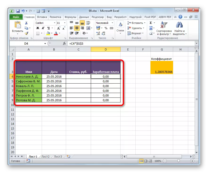
Let's see how the example you can form communication by direct binding. We have two tables on two sheets. On the same table, the salary is calculated using the formula by multiplying the employee rates for a single coefficient.

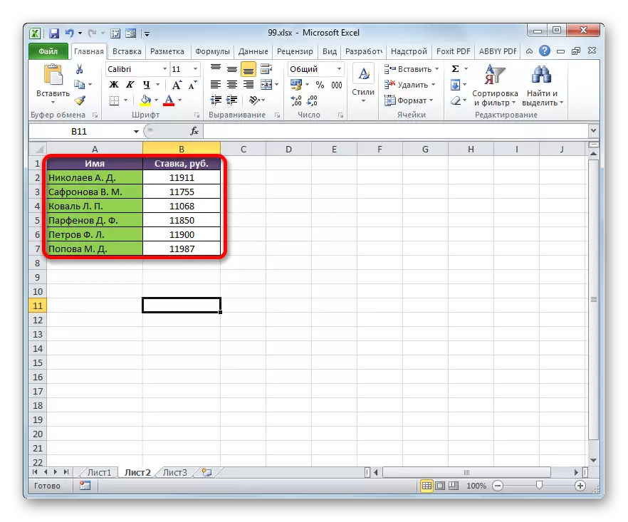
On the second sheet there is a table range in which there is a list of employees with their salary. The list of employees in both cases is presented in one order.

Table with employee rates in Microsoft Excel

It is necessary to make that data on the bets from the second sheet tighten into the corresponding cells of the first.

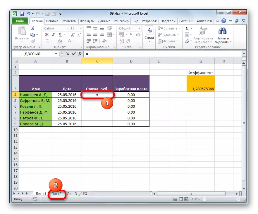
On the first sheet, we allocate the first cell of the "Bet" column. We put in it the sign "=". Next, click on the "Sheet 2" label, which is placed on the left part of the Excel interface over the status bar.

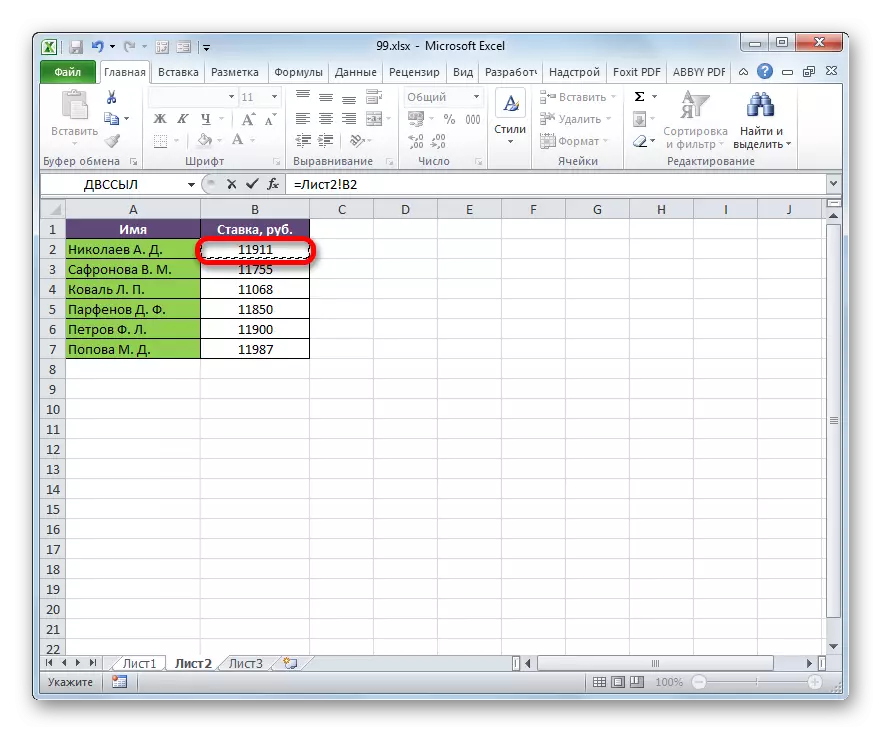
Go to the second sheet in Microsoft Excel

There is a movement in the second area of the document. Click on the first cell in the "Bet" column. Then click on the ENTER button on the keyboard to enter the data into the cell in which the "equal" sign was previously installed.

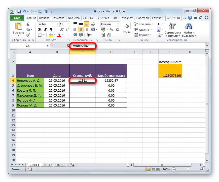
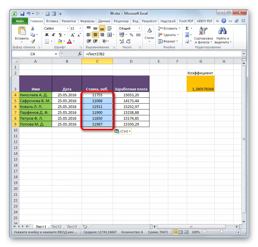
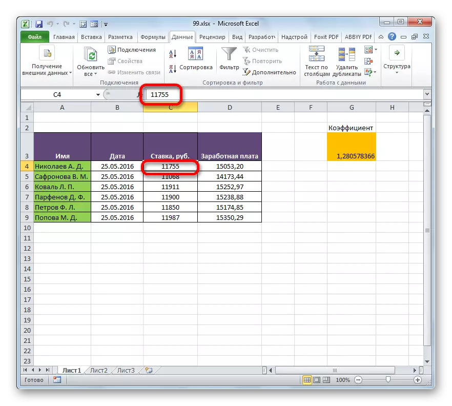
Binding with a cell of the second table in Microsoft Excel

Then there is an automatic transition to the first sheet. As we can see, the value of the first employee from the second table is pulled into the corresponding cell. By installing the cursor on a cell containing a bet, we see that the usual formula is used to display data on the screen. But in front of the coordinates of the cell, from where the data is output, there is an expression "list2!", Which indicates the name of the document area where they are located. The general formula in our case looks like this:
= List2! B2

Two cells of two tables are connected to Microsoft Excel

Now you need to transfer data about the rates of all other employees of the enterprise. Of course, this can be done in the same way that we fulfilled the task for the first employee, but considering that both employee lists are located in the same order, the task can be significantly simplified and accelerated by its decision. This can be done by simply by copying the formula to the range below. Due to the fact that the references to Excel are relative, when copying their values, the values shift are shifted that we need. The copy procedure itself can be made using a filling marker.
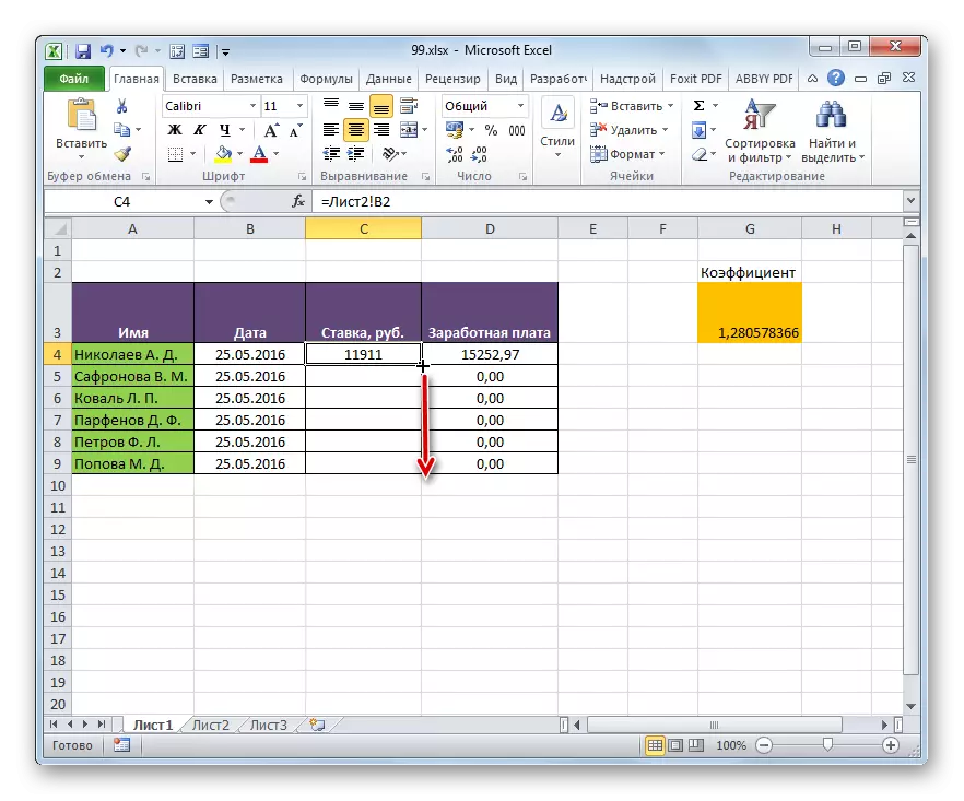
So, we put the cursor to the lower right area of the element with the formula. After that, the cursor must convert to the filling marker in the form of a black cross. We perform the clamp of the left mouse button and pull the cursor to the number of the column.

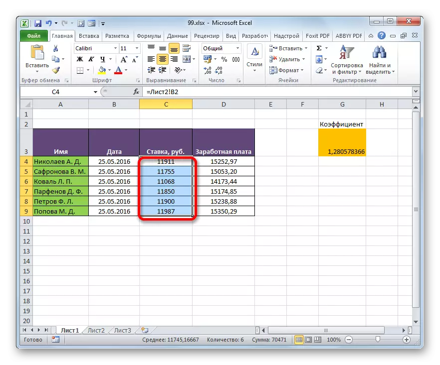
All data from a similar column on a sheet 2 were pulled into a table on a sheet 1. When the data changes on a sheet 2, they will automatically change on the first.

All columns of the second table column are transferred to the first in Microsoft Excel

Method 2: Using the Blundering of Operators Index - Search

But what to do if the list of employees in table arrays is not located in the same order? In this case, as stated earlier, one of the options is to install the relationship between each of those cells that should be associated manually. But it is suitable except for small tables. For massive ranges, this option will at best take a lot of time on the implementation, and at worst - in practice it will generally be unrealistic. But this problem can be solved using a bunch of operators index - search. Let's see how it can be done by tilling the data in the tables about which the conversation was in the previous method.

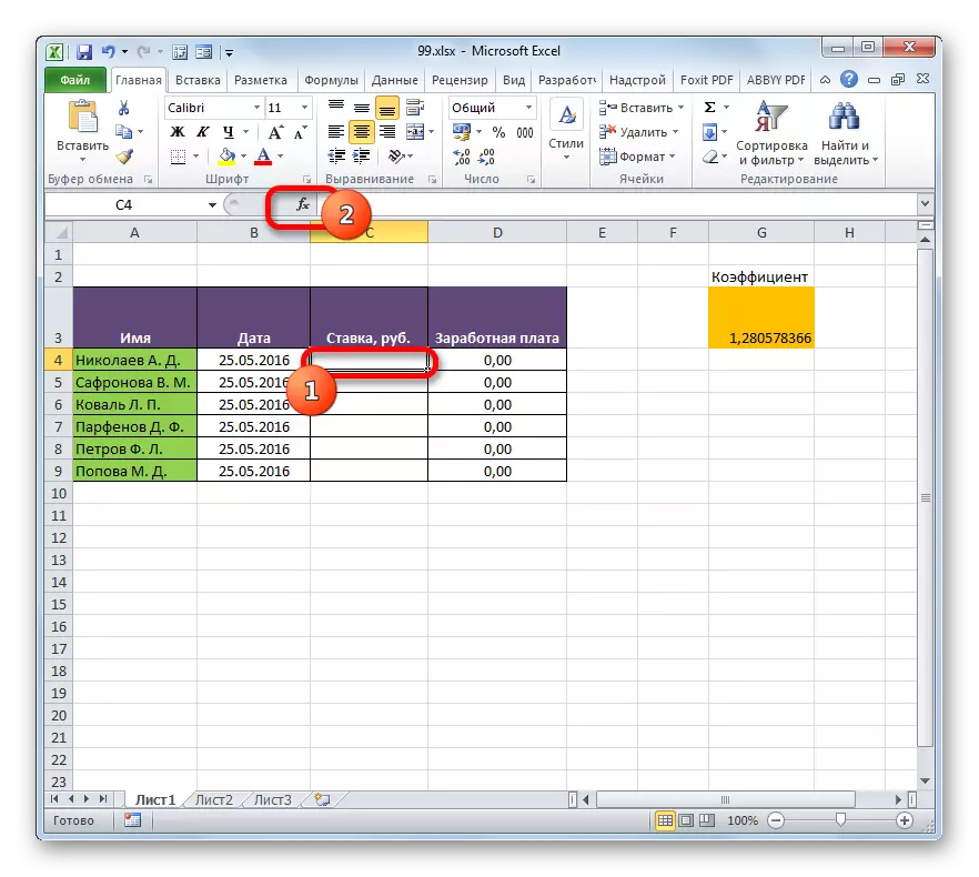
We highlight the first element of the "Bet" column. Go to the functions wizard by clicking on the "Insert function" icon.

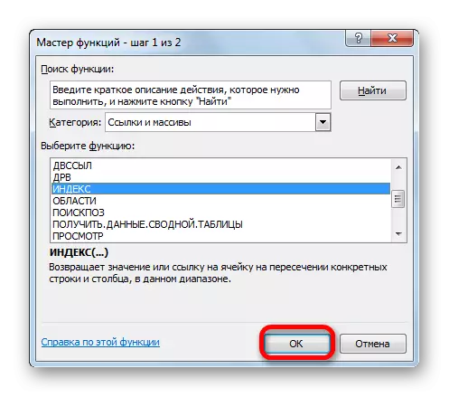
In the wizard of functions in the group "Links and arrays" we find and allocate the name "index".

Transition to the Argometheus window function index in Microsoft Excel

This operator has two forms: a form for working with arrays and reference. In our case, the first option is required, so in the next form selection window that opens, select it and click on the "OK" button.

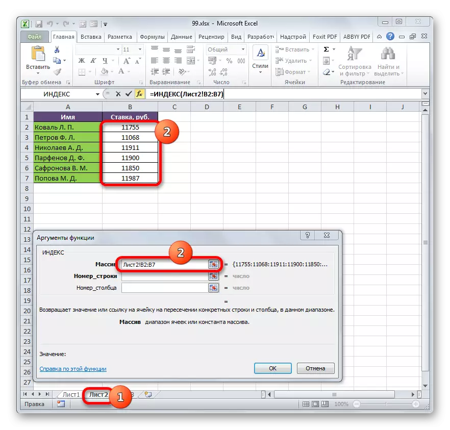
Select Function Function Index in Microsoft Excel

The operator's arguments index start running. The task of the specified function is the output of the value located in the selected range in the line with the specified number. General formula operator index such:
= Index (array; number_name; [number_stolbits])

The "array" is an argument containing the range of the range from which we will extract information by the number of the specified row.
"Row number" is an argument that is the number of this line. It is important to know that the line number should be specified not relative to the entire document, but only relative to the allocated array.
The "number of the column" is an argument that is optional. To solve the specifically of our task, we will not use it, and therefore it is not necessary to describe it separately.
We put the cursor in the "Array" field. After that, go to the sheet 2 and, holding the left mouse button, select the entire contents of the "rate" column.

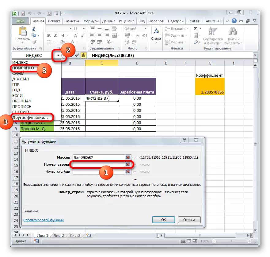
Argument Array in the Argument Window Function Index in Microsoft Excel

After the coordinates are displayed in the operator's window, we put the cursor in the "Row number" field. We will withdraw this argument using the search operator. Therefore, click on a triangle that is located on the left of the function string. A list of newly used operators opens. If you find the name "Search Company" among them, you can click on it. In the opposite case, click on the latest point of the list - "Other functions ...".

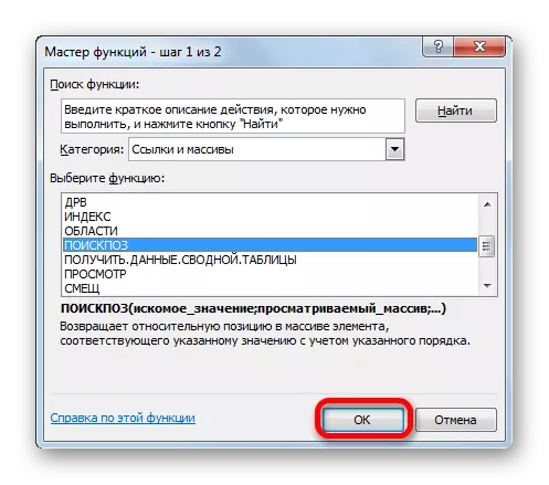
Argument window function index in Microsoft Excel

Standard window wizard window starts. Go to it in the same group "Links and arrays". This time in the list, choose the item "Search Company". Perform a click on the "OK" button.

Transition to the Arguamet window of the search function in Microsoft Excel

Activation of the arguments of the arguments of the search operator is performed. The specified function is designed to output the value number in a specific array by its name. It is thanks to this feature that we calculate the number of a string of a specific value for the function function. The syntax of the search board is presented:
= Search board (search_name; viewing__nassive; [type_station])
"The desired" is an argument containing the name or address of the cell of the third-party range in which it is located. It is the position of this name in the target range and should be calculated. In our case, the role of the first argument will be referenced to cells on a sheet 1, in which employees are located.
"Listful array" is an argument, which is a reference to an array, which performs the search for the specified value to determine its position. We will have this role to execute the address of the "Name" column on a sheet 2.
"Type of comparison" - an argument that is optional, but, unlike the previous operator, this optional argument will be needed. It indicates how to match the operator is the desired value with an array. This argument can have one of three values: -1; 0; 1. For disordered arrays, select the option "0". This option is suitable for our case.
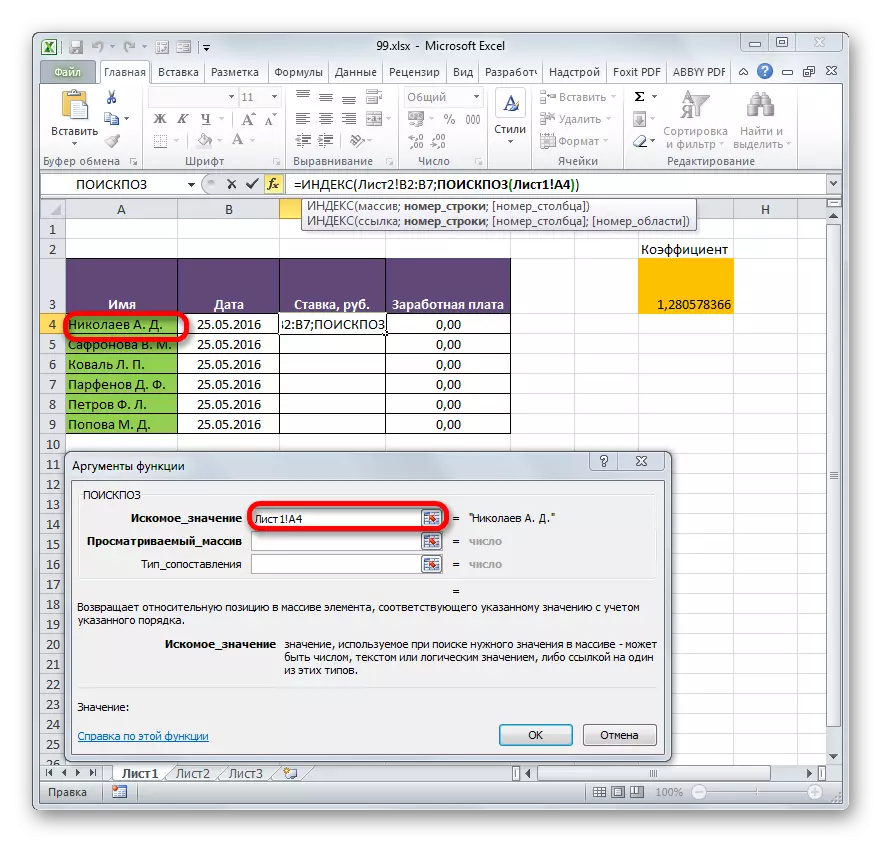
So, proceed to filling the argument window fields. We put the cursor in the field "Fogular value", click on the first cell "name" column on a sheet 1.

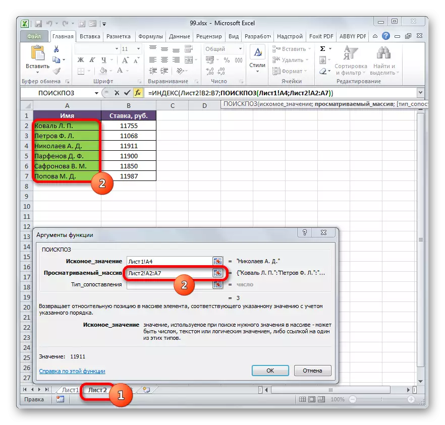
The argument is the desired value in the argument window of the search function in Microsoft Excel

After the coordinates are displayed, set the cursor in the "Listing Massive" field and go to the "Sheet 2" label, which is located at the bottom of the Excel window above the status bar. Clement the left mouse button and highlight the cursor all cells of the "Name" column.

The argument is viewed by an array in the argument window of the search function in Microsoft Excel

After their coordinates are displayed in the "Listing Massive" field, go to the "Mapping Type" field and set the number "0" from the keyboard. After that, we again return to the field "Looking through the Array". The fact is that we will perform copying the formula, as we did in the previous method. There will be a shift of addresses, but here the coordinates of the Array viewed we need to secure. He should not shift. We highlight the coordinates with the cursor and click on the F4 function key. As you can see, the dollar sign appeared before the coordinates, which means that reference from relative turned into absolute. Then click on the "OK" button.

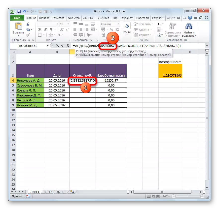
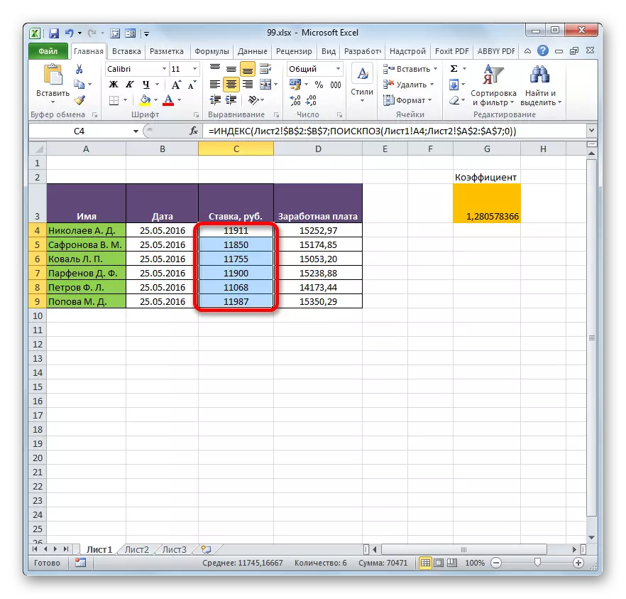
Arguamet window Functions for the search board in Microsoft Excel

The result is displayed in the first cell of the "Bet" column. But before copying, we need to fix another area, namely the first argument function index. To do this, select the column element, which contains a formula, and move to the formula string. Allocate the first argument of the operator index (B2: B7) and click on the F4 button. As you can see, the dollar sign appeared near the selected coordinates. Click the ENTER key. In general, the formula took the following form:
= Index (sheet2! $ B $ 2: $ b $ 7; search board (sheet1! A4; list2! $ A $ 2: $ A $ 7; 0))

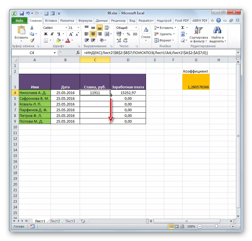
Convert links to absolute in Microsoft Excel

Now you can copy using a filling marker. We call it in the same way that we have spoken earlier, and stretch to the end of the tabular range.

As you can see, despite the fact that the order of strings in two related tables does not coincide, nevertheless, all values are tightened according to the names of workers. This was achieved thanks to the use of the combination of operators index search.

Values are associated due to a combination of functions of index expiration in Microsoft Excel

The amount of salary for the enterprise is recalculated in Microsoft Excel

Method 4: Special Insert

Tie table arrays in Excel can also be using a special insertion.

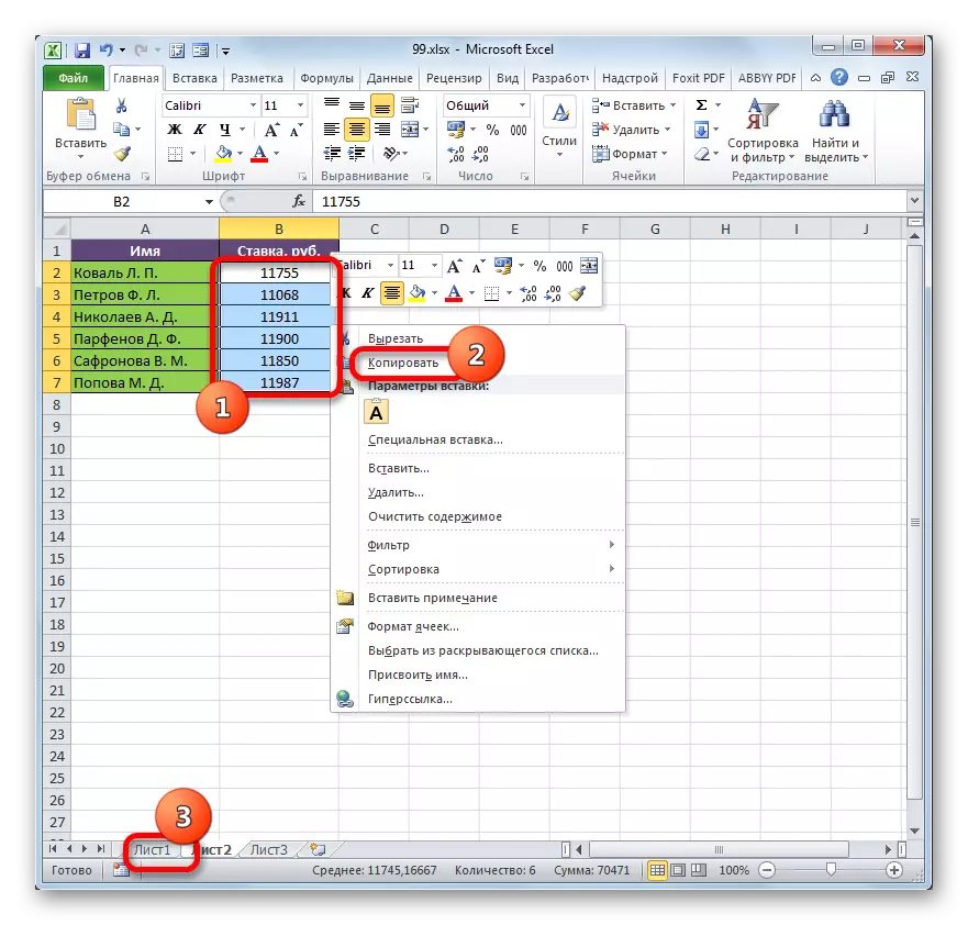
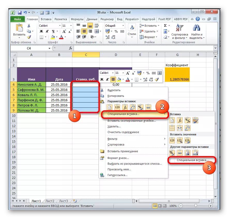
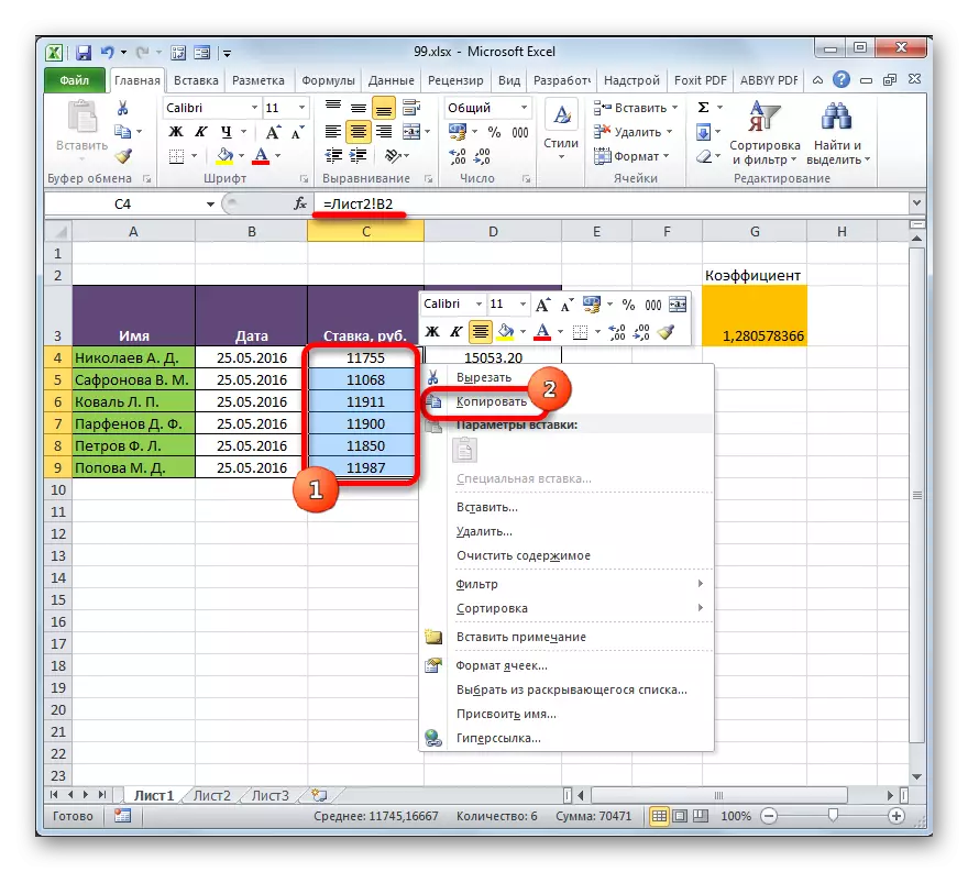
Select the values that you want to "tighten" to another table. In our case, this is the "Bet" column range on a sheet 2. Click on the dedicated fragment with the right mouse button. In the list that opens, select the "Copy" item. An alternative combination is the Ctrl + C key combination. After that, we move to the sheet 1.

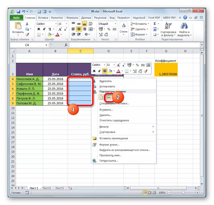
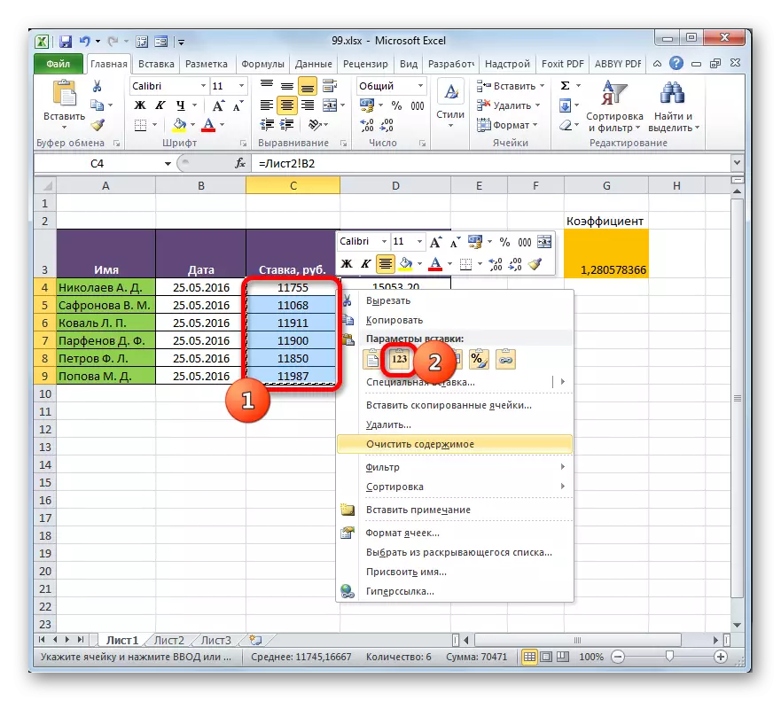
Moving to the area of the book you need, allocate the cells in which the values will need to be tightened. In our case, this is the "bid" column. Click on the dedicated fragment with the right mouse button. In the context menu in the "Insert parameters" toolbar, click on the "Insert Communication" icon.

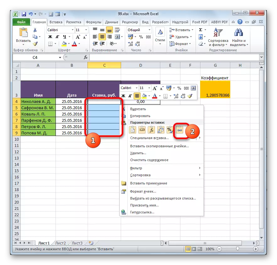
There is also an alternative. He, by the way, is the only one for older versions of Excel. In the context menu, we bring the cursor to the "Special Insert" item. In the additional menu that opens, select the position with the same name.

Transition to a special insert in Microsoft Excel

After that, a special insert window opens. Click on the "Insert communication" button in the lower left corner of the cell.

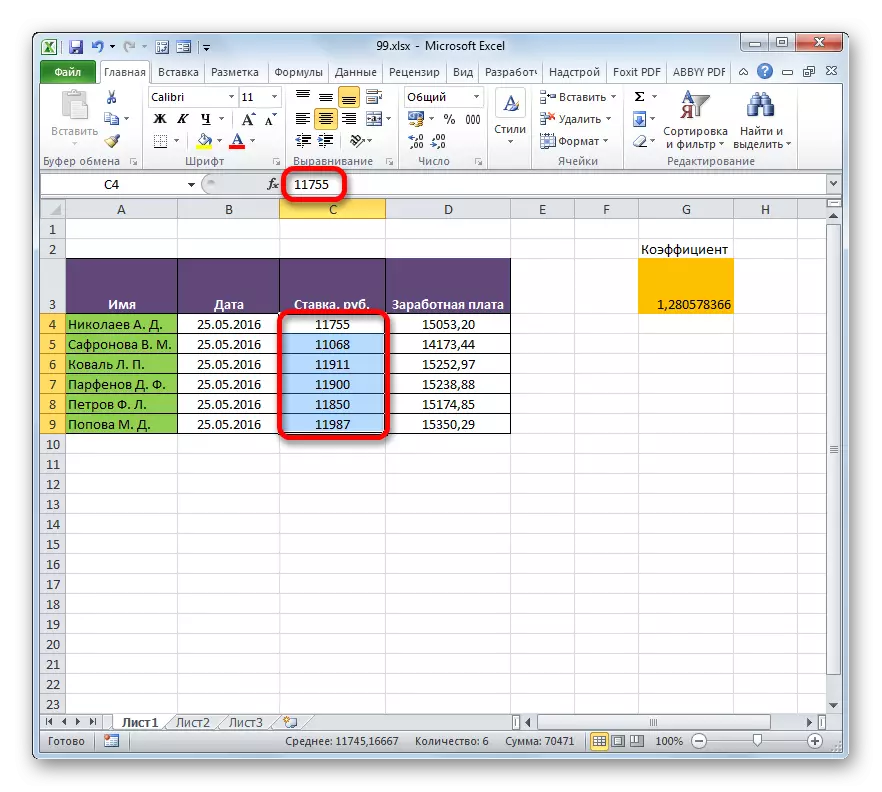
Special insert window in Microsoft Excel

Whatever option you choose, values from one table array will be inserted into another. When changing data in the source, they will also automatically change in the inserted range.

Values are inserted using a special insertion in Microsoft Excel

Lesson: Special insert in Excele

Method 5: Communication between tables in several books

In addition, you can organize a link between the table areas in different books. This uses a special insert tool. Actions will be absolutely similar to those we considered in the previous method, except that the navigation during the formulas will not have between the areas of one book, but between the files. Naturally, all related books should be opened.

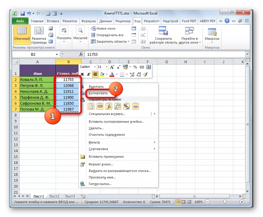
Select the data range to be transferred to another book. Click on it right mouse button and select the "Copy" position in the opened menu.

Copying data from the book in Microsoft Excel

Then we move to the book in which this data should be inserted. Select the desired range. Click right mouse button. In the context menu in the "Insert Settings" group, select the "Insert Communication" item.

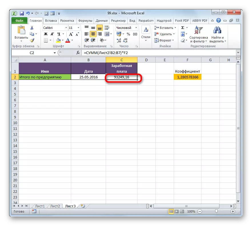
Insert communication from another book in Microsoft Excel

After that, the values will be inserted. When changing data in the source book, a table array from the working book will tighten them automatically. And it is not at all necessary to ensure that both books are open. It is enough to open one only workbook, and it will automatically tailage data from a closed related document if there were previous changes in it.

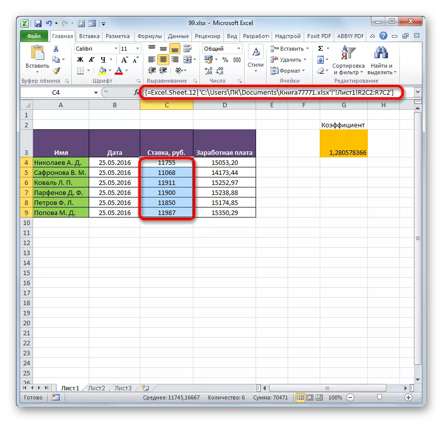
Communication from another book is inserted in Microsoft Excel

But it should be noted that in this case the inset will be produced in the form of an unchanged array. When trying to change any cell with the inserted data, a message will be populated informing about the inability to do this.

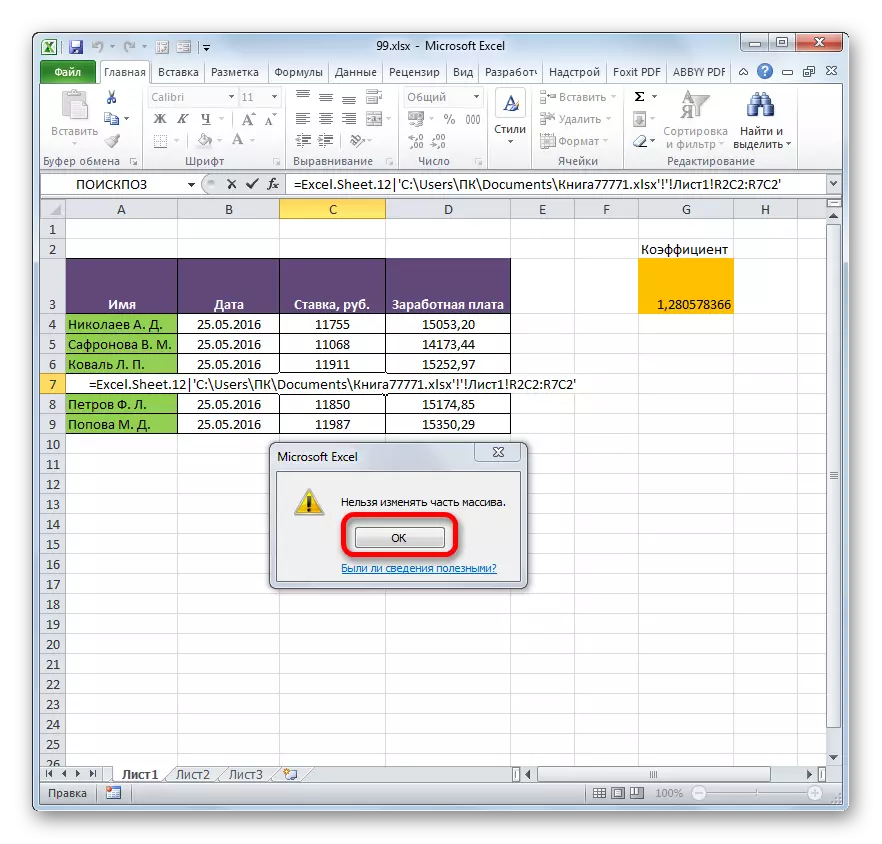
Changes in such an array associated with another book can only break the connection.

Title breaks between tables

Sometimes it is required to break the connection between the tables. The reason for this can be the above described when you want to change an array inserted from another book and simply the user's reluctance so that the data in the same table is automatically updated from the other.

Method 1: Communication breaks between books

To break the connection between books in all cells, by performing actually one operation. In this case, the data in the cells will remain, but they will already be static not updated values that do not depend on other documents.

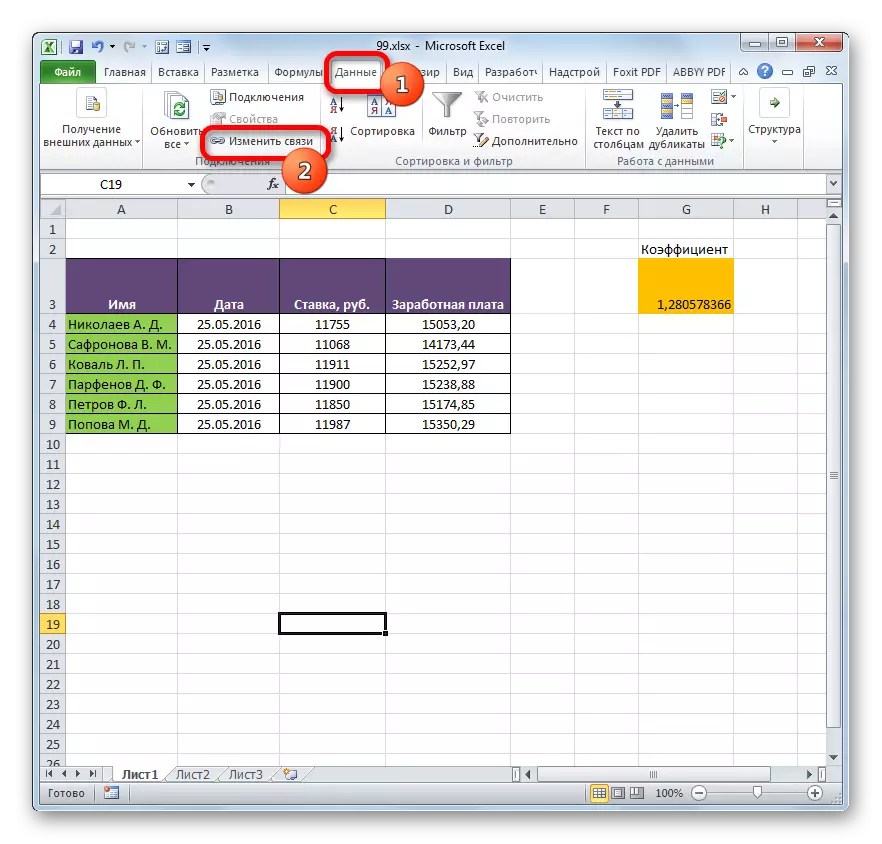
In the book in which values from other files are tightened, go to the Data tab. Click on the "Change links" icon, which is located on the tape in the "Connection" toolbar. It should be noted that if the current book does not contain connections with other files, then this button is inactive.

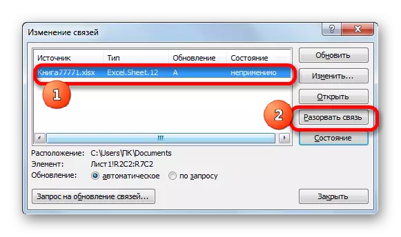
Transition to changes in links in Microsoft Excel

The link change window is launched. Select from the list of related books (if there are several of them) the file with which we want to break the connection. Click on the button "Break the connection".

An information window opens, which provides a warning about the consequences of further actions. If you are sure that you are going to do, click on the "Break Communication" button.

After that, all references to the specified file in the current document will be replaced with static values.

Links are replaced with static values in Microsoft Excel

Method 2: Inserting values

But the above method is suitable only if you need to completely break all the links between the two books. What if you need to disconnect the associated tables within the same file? You can do this by copying the data, and then inserting the same place as values. By the way, this method can be ruptied between the individual data ranges of various books without breaking a common relationship between files. Let's see how this method works in practice.

We highlight the range in which we wish to delete communication with another table. Click on it right mouse button. In the open menu, select the "Copy" item. Instead of the specified actions, you can dial an alternative combination of hot keys Ctrl + C.

Next, without removing the selection from the same fragment, again click on it with the right mouse button. This time in the list of action, click on the "Value" icon, which is posted in the Insert Parameters group.

After that, all references in the dedicated range will be replaced with static values.

As you can see, Excel has ways and tools to associate several tables among themselves. At the same time, tabular data can be on other sheets and even in different books. If necessary, this connection can be easily broken.