Comparison of tables in Excel

Quite often, Excel users have a task of comparing two tables or lists to identify differences in them or missing items. Each user copes with this task in its own way, but most often a rather large amount of time is spent on solving the specified question, since not all approaches to this problem are rational. At the same time, there are several proven actions algorithms that will allow compare lists or table arrays in fairly short time with minimal considerable effort. Let's consider details these options.

In the same way, you can compare the data in the tables that are located on different sheets. But in this case, it is desirable that the lines in them are numbered. The rest of the comparison procedure is almost exactly the same as described above, besides the fact that when making the formula, it is necessary to switch between sheets. In our case, the expression will have the following form:

= B2 = List2! B2

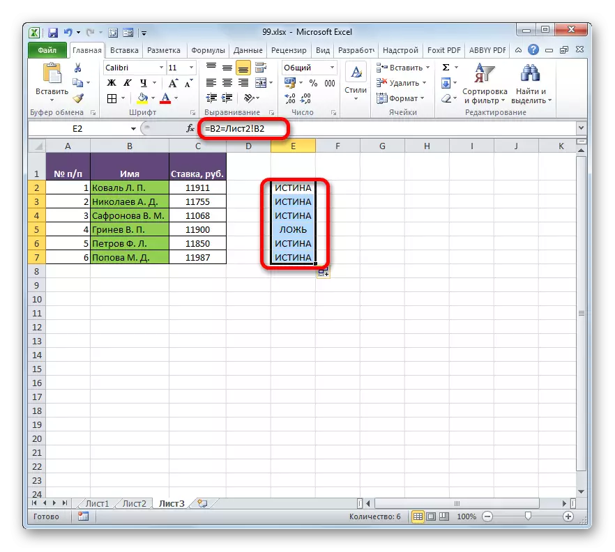
That is, as we see, in front of the data coordinates, which are located on other sheets other than where the comparison result is displayed, the sheet number and an exclamation mark is indicated.

Method 2: Selection of groups of cells

Comparison can be made using the tool for the separation of groups of cells. With it, you can also compare only synchronized and ordered lists. In addition, in this case, lists must be located next to each other on one sheet.

1. Select compared arrays. Go to the "Home" tab. Next, click on the "Find and Select" icon, which is located on the tape in the Editing toolbar. There is a list in which you should select the position "Selection of the group of cells ...".

   

   In addition, the selection of the group of cells can be reached in another way. This option will especially be useful to those users who have the version of the program earlier than Excel 2007, since the method via the "Find and Select" button does not support these applications. Select arrays that wish to compare, and click on the F5 key.

2. A small transition window is activated. Click on the button "highlight ..." in its lower left corner.



3. After that, whatever two of the above options you have elected, the selection window of cell groups is launched. Install the switch to the "highlight on line" position. Click on the "OK" button.



4. As we can see, after that, the inconsistent values ​​of the lines will be highlighted with a different tint. In addition, how can be judged from the contents of the formula line, the program will make an active one of the cells in the indicated non-coincided lines.

Method 3: Conditional Formatting

You can make a comparison by applying conditional formatting method. As in the previous method, compared areas should be on a single Excel working sheet and be synchronized with each other.

1. First of all, we choose what tabular region will be considered the main, and in what to look for the difference. Last let's do in the second table. Therefore, we allocate a list of workers in it. Moving to the "Home" tab, click on the "Conditional Formatting" button, which has a location on the tape in the "Styles" block. From the drop-down list, go through the "Rules Management" item.



2. The rules manager dispatcher window is activated. We click on it to the "Create Rule" button.



3. In the running window, we select the "use formula" position. In the "Format Cell" field, write a formula containing the addresses of the first cells of the ranges of compared columns, separated by the "not equal" sign (). Just before this expression this time will stand the sign "=". In addition, to all column coordinates in this formula, you need to apply an absolute addressing. To do this, we allocate the formula with the cursor and click on the F4 key three times. As we can see, the dollar sign appeared near all the column addresses, which means turning the links to absolute. For our particular case, the formula will take the following form:

   = $ A2 $ D2

   We record this expression in the above field. After that, we click on the "Format ..." button.



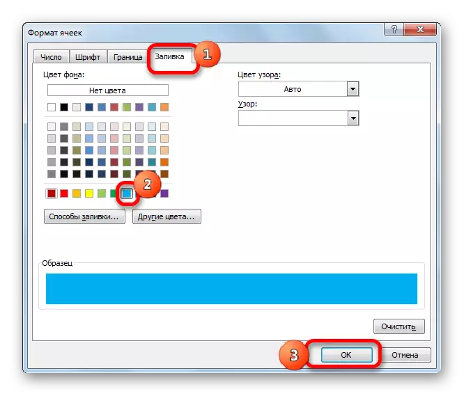
4. The "Cell format" window is activated. We go to the "Fill" tab. Here in the list of colors stop the choice on the color, which we want to paint those elements where data will not match. Click on the "OK" button.



5. Returning to the formatting rule window, click on the "OK" button.



6. After automatic moving to the "Rules Manager" window, click on the "OK" button and in it.



7. Now in the second table, elements that have data that are inconsistent with the corresponding values ​​of the first table area will be highlighted in the selected color.

There is another way to apply conditional formatting to perform the task. Like the previous options, it requires the location of both compared areas on one sheet, but in contrast to the previously described methods, the synchronization condition or sorting data will not be compulsory, which distinguishes this option from previously described.

1. We produce the selection of areas you need to compare.



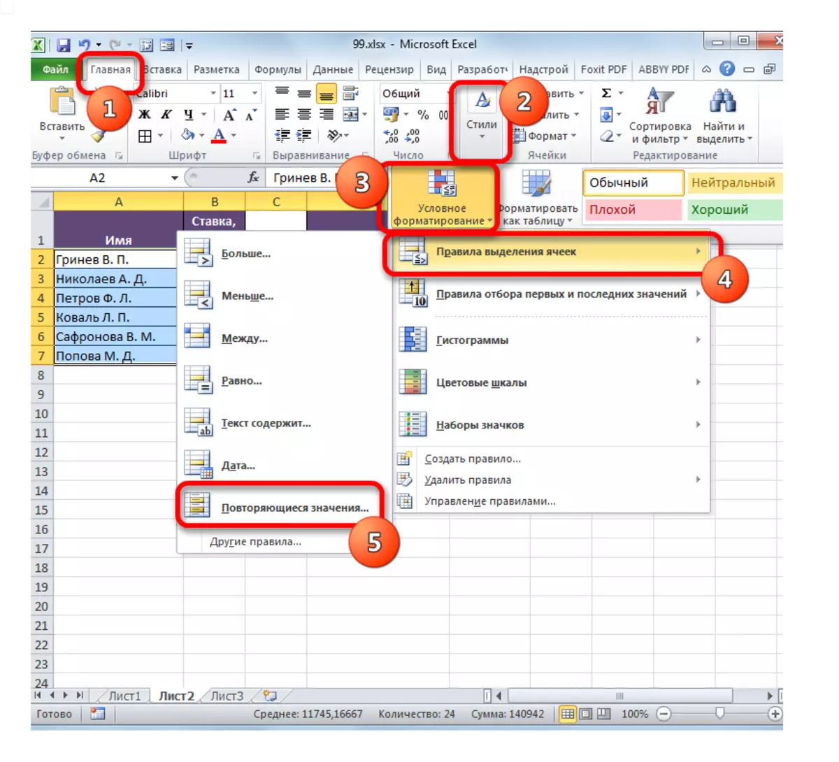
2. We carry out the transition to the tab called "Home". We click on the "Conditional Formatting" button. In the activated list, select the position "Rules for the allocation of cells". In the next menu, make the "Repeating Values" position.



3. The duplicate values ​​are launched. If you are all done correctly, then in this window it remains only to click on the "OK" button. Although, if you wish, in the appropriate field of this window, you can choose another color of the selection.



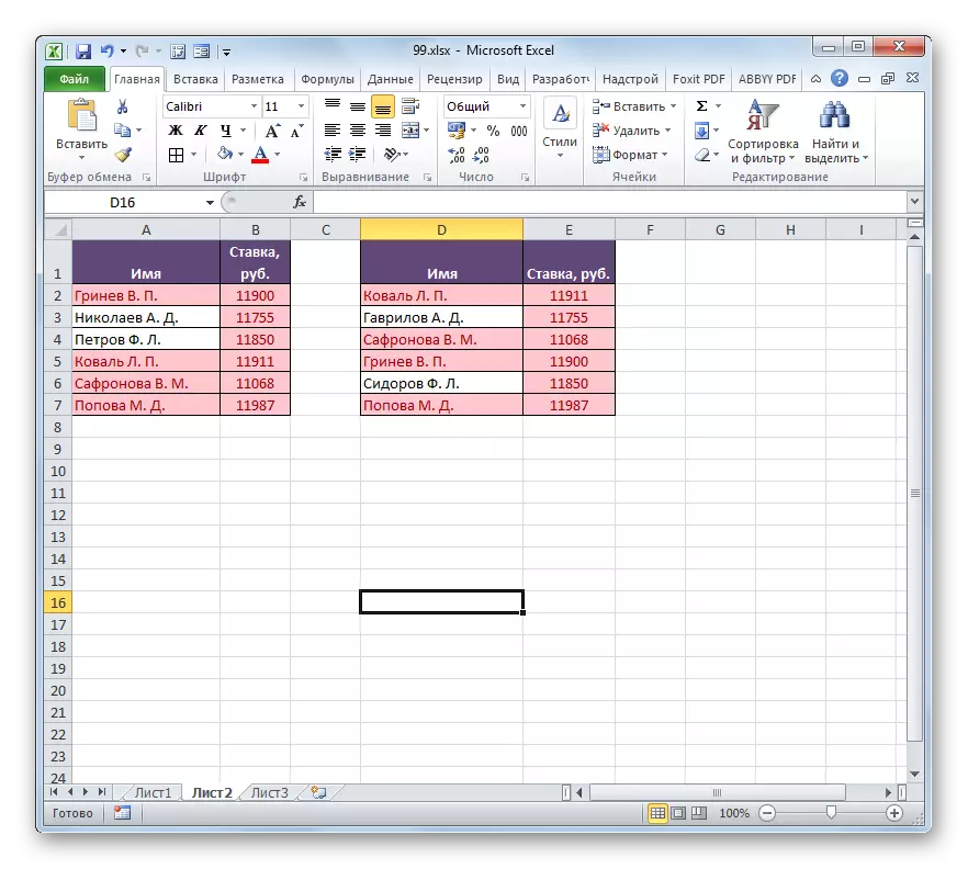
4. After we produce the specified action, all repetitive elements will be highlighted in the selected color. Those elements that do not coincide will remain painted in their original color (by default white). Thus, you can immediately see visually to see what the difference between arrays.

If you wish, you can, on the contrary, paint the inconsistent elements, and the indicators that match, leave with the fill of the previous color. At the same time, the algorithm of action is almost the same, but in the settings of the duplicate values ​​in the first field, instead of the "Repeated" parameter, select the "Unique" parameter. After that click on the "OK" button.

Thus, it is precisely those indicators that do not coincide.

Lesson: Conditional Formatting in Excel

Method 4: Comprehensive Formula

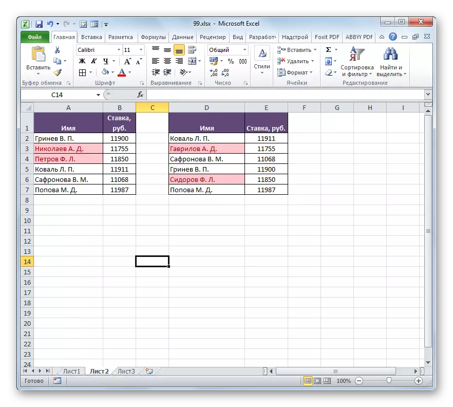
Also compare data with the help of a complex formula, the basis of which is the function of the meter. Using this tool, you can calculate how much each element from the selected column of the second table is repeated in the first.

The operator councils refers to the statistical group of functions. Its task is to count the number of cells, the values ​​in which satisfy the specified condition. The syntax of this operator has this kind:

= Schedules (Range; Criterion)

The argument "range" is the address of the array, which calculates the coincident values.

The argument "Criteria" specifies the condition of the coincidence. In our case, it will be the coordinates of the specific cells of the first tabular area.

1. We allocate the first element of the additional column in which the number of matches will be calculated. Next, click on the "Insert function" icon.



2. The functions wizard starts. Go to category "Statistical". Find in the list the name "countecles". After its selection, click on the "OK" button.



3. The operator arguments window started running. As we see, the names of the fields in this window correspond to the names of the arguments.

   Install the cursor in the "Range" field. After that, by holding the left mouse button, allocate all the values ​​of the column with the names of the second table. As you can see, the coordinates immediately fall into the specified field. But for our purposes, this address should be made by absolute. To do this, highlight the coordinates in the field and click on the F4 key.

   As you can see, the reference took the absolute form, which is characterized by the presence of dollar signs.

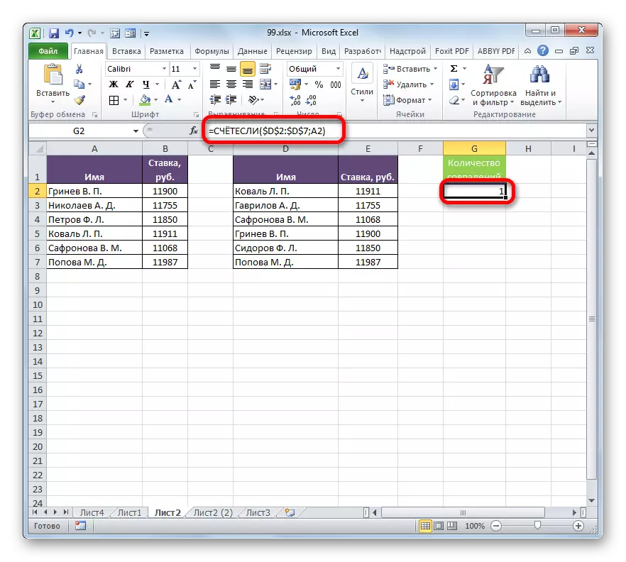
   Then go to the "Criterion" field by installing the cursor. Click on the first element with the last names in the first tabular range. In this case, leave the link relative. After it is displayed in the field, you can click on the "OK" button.



4. The result is output to the sheet element. It is equal to the number "1". This means that in the list of names of the second table, the name "Grinev V. P.", which is the first in the list of the first table array, occurs once.



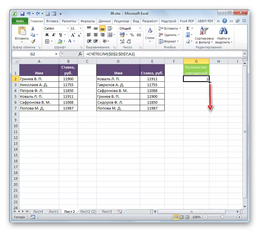
5. Now we need to create a similar expression and for all other elements of the first table. To do this, I will perform copying, using the filling marker, as we have already done before. We put the cursor to the bottom right part of the leaf element, which contains the function of the meter, and after converting it to the filling marker, clamp the left mouse button and pull the cursor down.



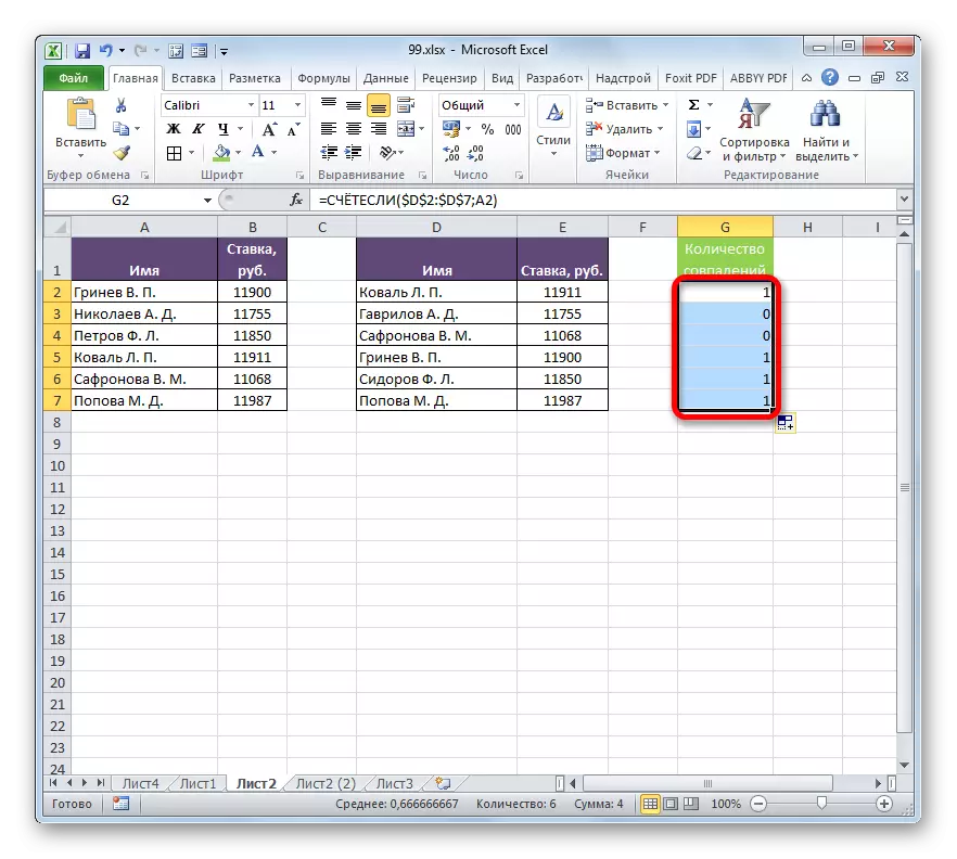
6. As we can see, the program has made a computation of coincidences, comparing each cell of the first table with data, which are located in the second table range. In four cases, the result was "1", and in two cases - "0". That is, the program could not find the two values ​​in the second table that are available in the first table array.

Of course, this expression in order to compare table indicators, it is possible to apply in the existing form, but it is possible to improve it.

We will make that the values ​​that exist in the second table, but are not available in the first, were displayed as a separate list.

1. First of all, we recycle our formula, but we will make it one of the operator's arguments if. To do this, we highlight the first cell in which the operator is the operator. In the formula string in front of it, we add the expression "if" without quotes and open the bracket. Further, so that it was easier for us to work, allocate the formulas in the formula row and click on the "Insert function" icon.



2. The function arguments window opens if. As you can see, the first window of the window has already been filled with the valuation of the operator's council. But we need to add something else in this field. We set there the cursor and the already existing expression add "= 0" without quotes.

   After that, go to the "Meaning if truth" field. Here we will use another nested function - line. Enter the word "string" without quotes, then open brackets and indicate the coordinates of the first cell with the surname in the second table, after which we close brackets. Specifically, in our case in the "Meaning if true" field, the following expression happened:

   Row (D2)

   Now the operator string will report functions if the line number in which the specific surname is located, and in the case when the condition specified in the first field will be performed, the function if this number will be displayed. Click on the "OK" button.



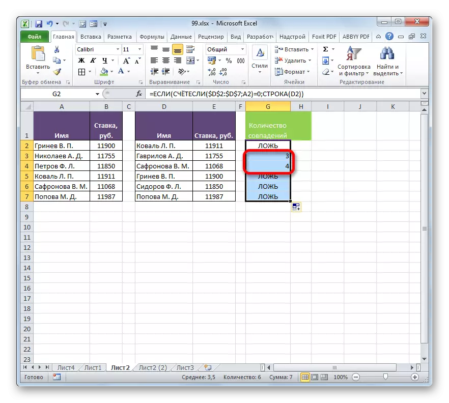
3. As you can see, the first result is displayed as "lies". This means that the value does not satisfy the conditions of the operator if. That is, the first surname is present in both lists.



4. Using the filling marker, which is already familiar to copy the expression of the operator if on the entire column. As we see, in two positions that are present in the second table, but not in the first, the formula issues rows numbers.



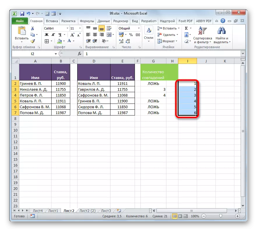
5. We retreat from the table area to the right and fill in the number column in order, starting from 1. The number of numbers must match the number of rows in the second compaable table. To speed up the numbering procedure, you can also use the fill marker.



6. After that, we highlight the first cell to the right of the speaker with the numbers and click the "Insert function" icon.



7. Wizard opens. Go to the category "Statistical" and produce the name of the "smallest" name. Click on the "OK" button.



8. The function is the smallest, the arguments of the arguments of which was disclosed, is intended to withdraw the specified smallest value.

   In the "Array" field, you should specify the coordinates of the range of the optional column "The number of matches", which we previously transformed using the function if. We make all links absolute.

   In the "k" field, it is indicated which in the account the smallest value should be displayed. Here we indicate the coordinates of the first cell of the column with the numbering, which we recently added. Address Leave relative. Click on the "OK" button.



9. The operator displays the result - number 3. It is precisely the smallest of the numbering of the inconsistent lines of table arrays. Using the filling marker, copy the formula to the nose itself.



10. Now, knowing the numbers of the rows of the incomprehensive elements, we can insert into the cell and their values ​​using the index function. Select the first element of the sheet containing the formula is the smallest. After that, go to the line formulas and before the name of the "smallest" add the name "index" without quotes, immediately open the bracket and put a point with a comma (;). Then we allocate the formula name "index" in the line and click on the "Paste Function" icon.



11. After that, a small window opens, in which it is necessary to determine if the reference view should have an index function or designed to work with arrays. We need a second option. It is installed by default, so that in this window simply click on the "OK" button.



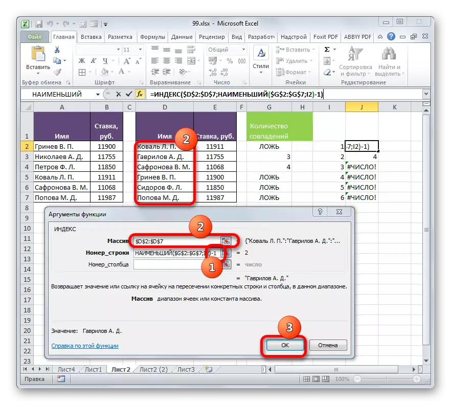
12. The argument window is running the index function. This operator is designed to output a value that is located in a specific array in the specified line.

    As you can see, the "Row number" field is already filled with the meaning values ​​of the smallest function. From an existing value there, the difference between the numbering of the Excel sheet and the internal numbering of the tabular region. As we see, we only have a hat on the table values. This means that the difference is one line. Therefore, add "-1" without quotes in the "Row number" field.

    In the "Array" field, specify the address of the value of the second table values. At the same time, all the coordinates make absolute, that is, we put the dollar sign before the method described by us.

    Click on the "OK" button.



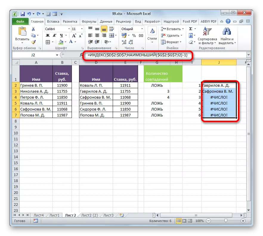
13. After withdrawing, the result on the screen is stretching the function using the fill marker to the end of the column down. As we see, both surnames that are present in the second table, but are not available in the first, are removed in a separate range.

Method 5: Comparison of arrays in different books

When comparing the ranges in different books, you can use the above methods, excluding those options where the placement of both tabular areas on one sheet is required. The main condition for the comparison procedure in this case is the opening of the windows of both files at the same time. For versions of Excel 2013 and later, as well as for versions to Excel 2007, there are no problems with the implementation of this condition. But in Excel 2007 and Excel 2010 in order to open both windows at the same time, additional manipulations are required. How to do it tells in a separate lesson.

Lesson: how to open Excel in different windows

As you can see, there are a number of possibilities to compare tables with each other. What kind of option to use depends on where the table data relative to each other is located (on one sheet, in different books, on different sheets), as well as from the user wants this comparison to be displayed on the screen.