

Quite often, you need to calculate the final result for various combinations of input data. Thus, the user will be able to evaluate all possible action options, select those, the result of the interaction of which it satisfies, and, finally, choose the most optimal option. In Excel, there is a special tool to perform this task - "Data Table" ("Substitution Table"). Let's find out how to use them to perform the above scenarios.
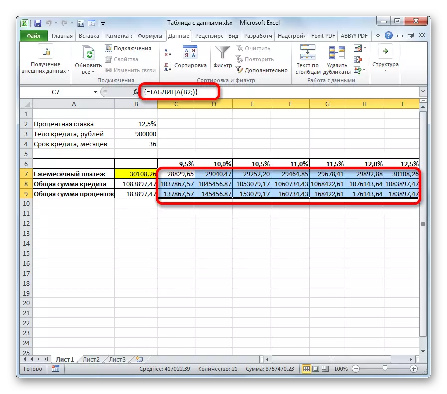
In addition, it can be noted that the amount of monthly payment at 12.5% per annum obtained as a result of the application of the substitution table corresponds to the value at the same amount of interest that we received by applying the PL function. This once again proves the correctness of the calculation.

After analyzing this table array, it should be said that, as we see, only at a rate of 9.5% per annum it turns out an acceptable level of monthly payment (less than 29,000 rubles).

Lesson: Calculation of annuity pay in Excel
Method 2: Using a tool with two variables
Of course, to find banks currently, which give a loan under 9.5% per annum, is very difficult, if at all really. Therefore, let's see what options exist in an acceptable level of the monthly payment at various combinations of other variables: the magnitude of the body of the loan and credit period. At the same time, the interest rate will be left unchanged (12.5%). In solving this task, we will help the "Data Table" tool using two variables.
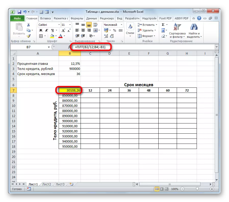
- Blacksmith new tabular array. Now in the names of the columns will be indicated a credit period (from 2 to 6 years in months in a step of one year), and in lines - the magnitude of the body of the loan (from 850,000 to 950000 rubles with a step of 10,000 rubles). In this case, the mandatory condition is that the cell, in which the calculation formula is located (in our case, PLT) was located on the border of the names of rows and columns. Without performing this condition, the tool will not work when using two variables.
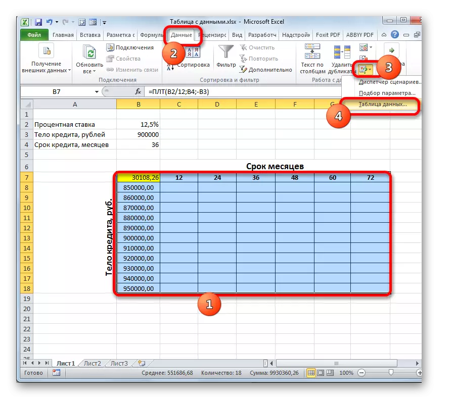
- Then we allocate the entire table range, including the name of columns, rows and cells with the PLT formula. Go to the "Data" tab. As in the previous time, click on the "Analysis" What if "", in the "Working with Data" toolbar. In the list that opens, select the "Data Table ...".
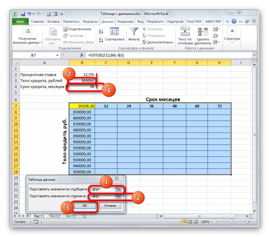
- The "Data Table" tool window starts. In this case, we will need both fields. In the "Substitution Values on columns in" field, indicate the coordinates of the cell containing the loan period in the primary data. In the "Substitution Values via" field, specify the address of the cell of the source parameters containing the value of the body of the loan. After all data is entered. Clay on the "OK" button.
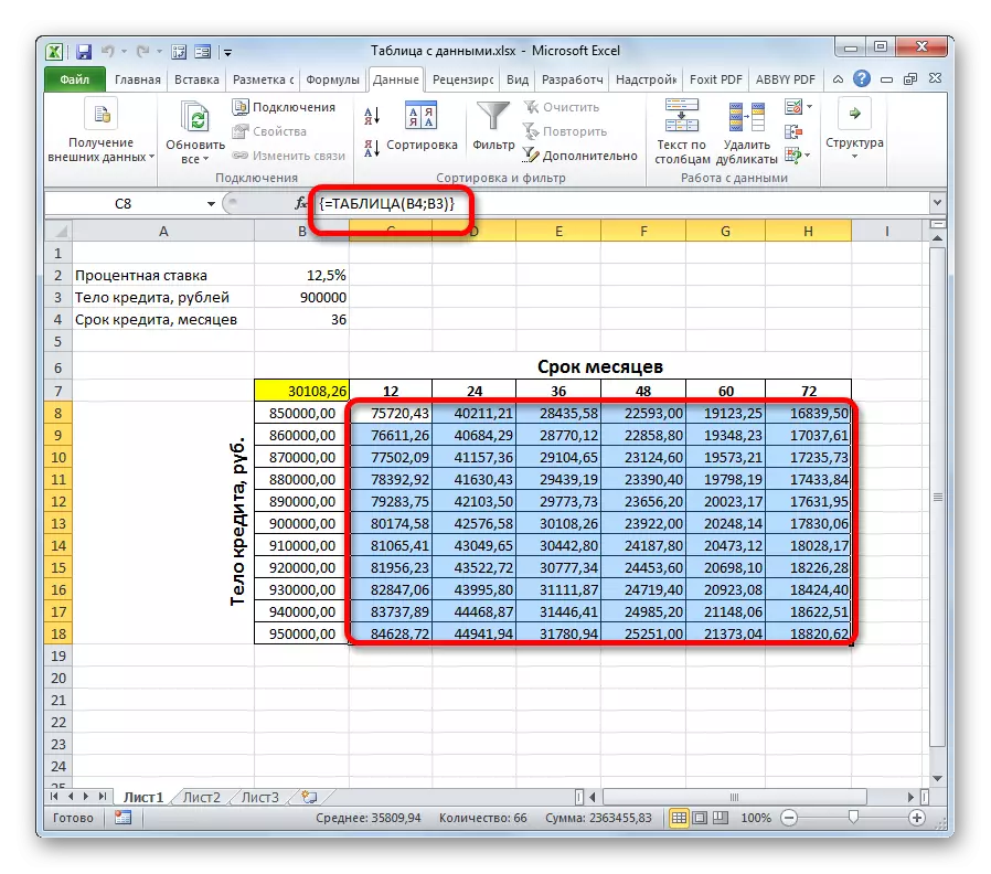
- The program performs the calculation and fills the tabular data range. At the intersection of rows and columns, you can now observe what will be the monthly payment, with the corresponding value of annual percent and the specified loan period.
- As you can see, quite a lot of values. To solve other tasks, there may be even more. Therefore, to make the issuance of the results more visual and immediately determine which values do not satisfy the specified condition, you can use visualization tools. In our case, it will be conditional formatting. We highlight all the values of the table range, excluding the headers of the rows and columns.
- We move to the "Home" tab and clay on the "Conditional Formatting" icon. It is located in the "Styles" tools block on the ribbon. In the discontinuing menu, select the item "Rules for the allocation of cells". In the additional list of clicking on the position "less ...".
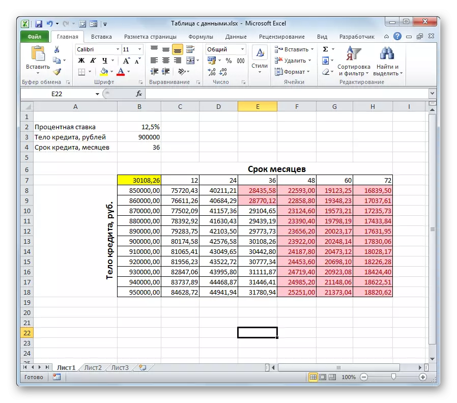
- Following this, the conditional formatting setting window opens. In the left field, we specify the amount less than which cells will be highlighted. As you remember, we satisfy us at which the monthly loan payment will be less than 29,000 rubles. Enter this number. In the right field, it is possible to select the selection color, although you can leave it by default. After all the required settings are entered, clay on the "OK" button.
- After that, all cells, the values in which correspond to the condition described above will be highlighted by color.


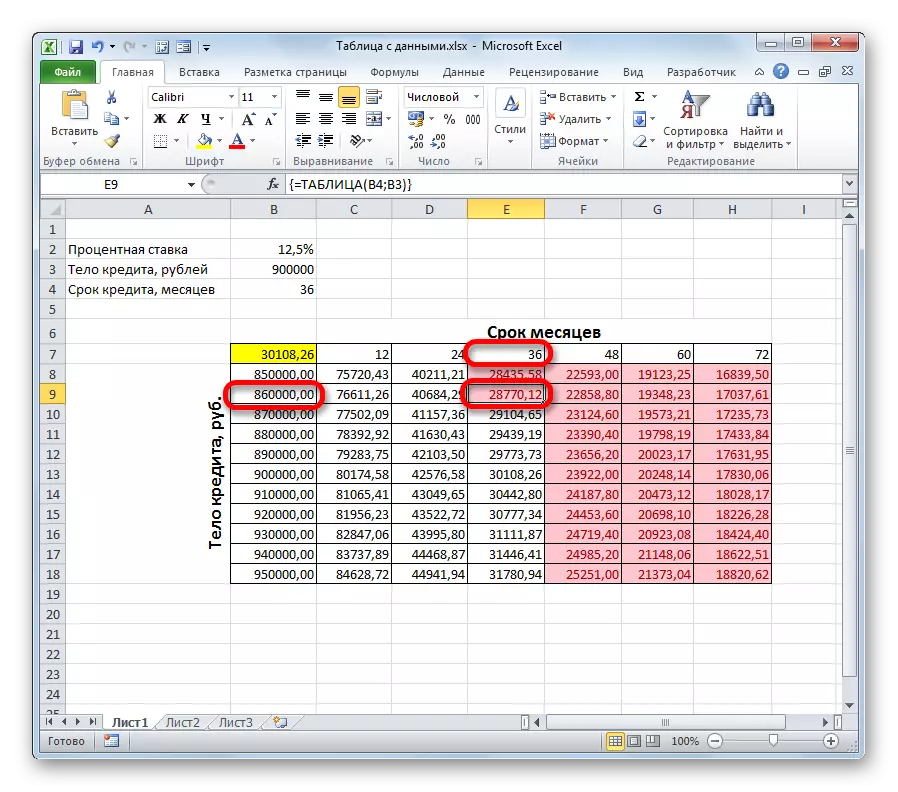
After analyzing the table array, you can make some conclusions. As you can see, with the current lending time (36 months) to invest in the above-mentioned amount of the monthly payment, we need to take a loan that does not exceed 80,000.00 rubles, that is, 40,000 is less than originally planned.
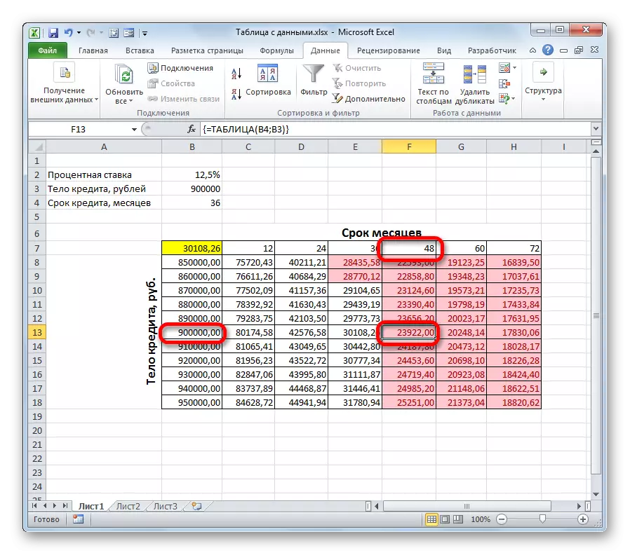
If we still intend to take a loan of 900,000 rubles, the credit period should be 4 years (48 months). Only in this case, the size of the monthly payment will not exceed the established boundary of 29,000 rubles.
Thus, using this table array and analyzing "for" and "against" each option, the borrower can take a specific decision on lending conditions by choosing the most response option from all possible.
Of course, the substitution table can be used not only to calculate credit options, but also to solve a plurality of other tasks.
Lesson: Conditional Formatting in Excel
In general, it should be noted that the substitution table is a very useful and relatively simple tool to determine the result with various combinations of variables. Applying both conditional formatting simultaneously with it, in addition, you can visualize the information received.