How to make a calculator in Excel

For permanent users, Excel is no secret that in this program you can produce various mathematical, engineering and financial calculations. This feature is implemented by applying various formulas and functions. But, if Excel is constantly used to carry out such calculations, the question of the organization necessary for this tools is relevant directly on the sheet, which will significantly increase the calculation speed and the level of convenience for the user. Let's find out how to make a similar calculator in Excel.

Calculator creation procedure

A particularly pressing given task becomes in case of need to constantly carry out the same type of calculations and calculations associated with a certain type of activity. In general, all calculators in Excel can be divided into two groups: universal (used for general mathematical calculations) and narrow-profile. The last group is divided into many types: engineering, financial, credit investment, etc. It is from the functionality of the calculator, first of all, the choice of the algorithm for its creation depends.

Method 1: Use macros

First of all, consider the algorithms for creating custom calculators. Let's start with the creation of the simplest universal calculator. This tool will perform elementary arithmetic actions: addition, multiplication of subtraction, division, etc. It is implemented using a macro. Therefore, before proceeding with the procedure for creating, you need to make sure that you have enabled macros and developer panel. If it is not so, then you must activate the work of macros.

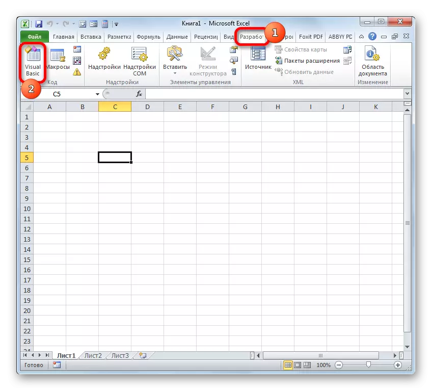
1. After the above presets are made, move to the "Developer" tab. We click on the "Visual Basic" icon, which is located on the tape in the "Code" toolbar.



2. The VBA Editor window starts. If the central area is displayed in gray, and not white, then it means that the field of the input of the code is absent. To turn on its display, go to the "View" menu item and click on the "Code" inscription in the list that appears. You can, instead of these manipulations, press the F7 function key. In any case, the Code input field will appear.



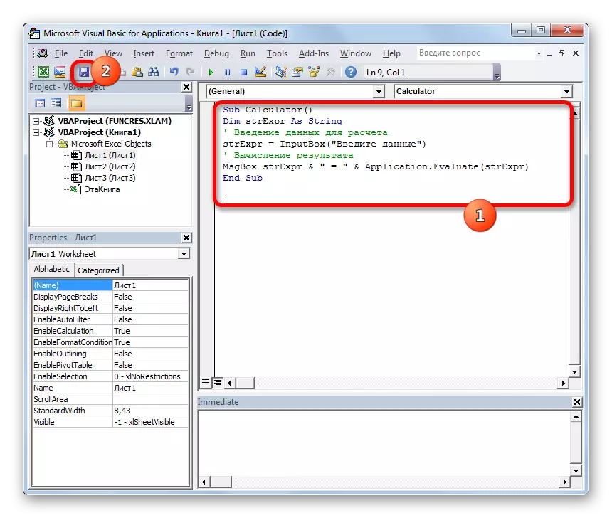
3. Here in the central region we need to write the macro code itself. It has the following form:

   Sub calculator ()

   Dim Strexpr AS String

   'Entering data for calculation

   STREXPR = INPUTBOX ("Enter Data")

   'Calculation of the result

   MSGBOX STREXPR & "=" & Application.evaluate (StrexPR)

   End Sub.

   Instead of the phrase "Enter Data" you can burn any other more acceptable for you. It is it that will be located above the field of expression.

   After the code is entered, the file must be overwritten. At the same time, it should be saved in the format with macros support. We click on the icon in the form of a floppy disk on the VBA editor toolbar.



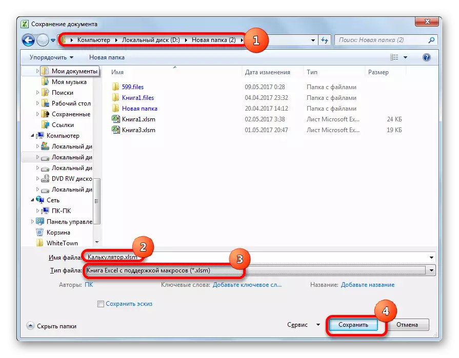
4. A document saving window is launched. Go to the directory on the hard disk or removable media where we want to save it. In the "File Name" field, you assign any desired name or leave the default that is assigned to it. In mandatory in the File Type field, select the name "Excel Book with Macros Support (* .xlsm)" from all available formats. After this step, clay on the "Save" button at the bottom of the window.



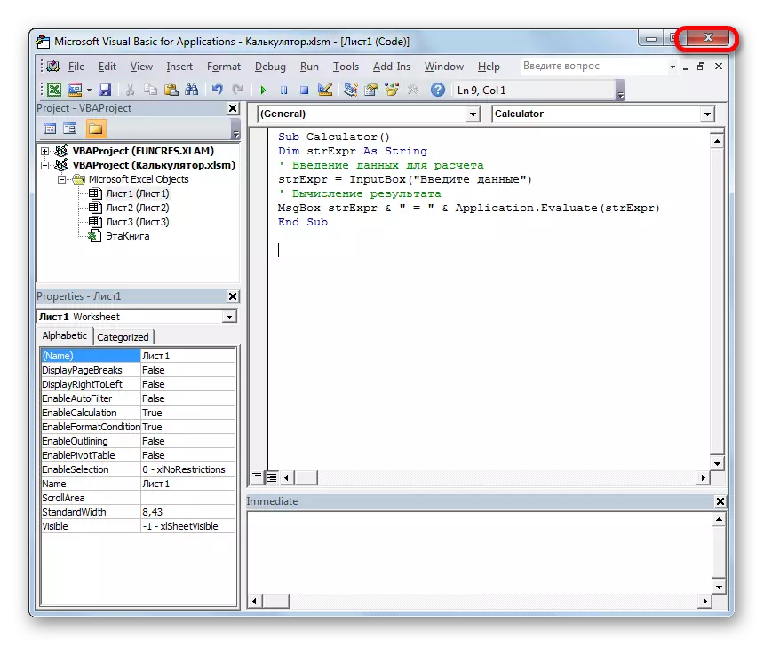
5. After that, you can close the macro editor window simply by clicking on the standard closing icon in the form of a red square with a white cross in its upper right corner.



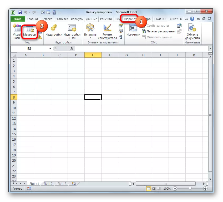
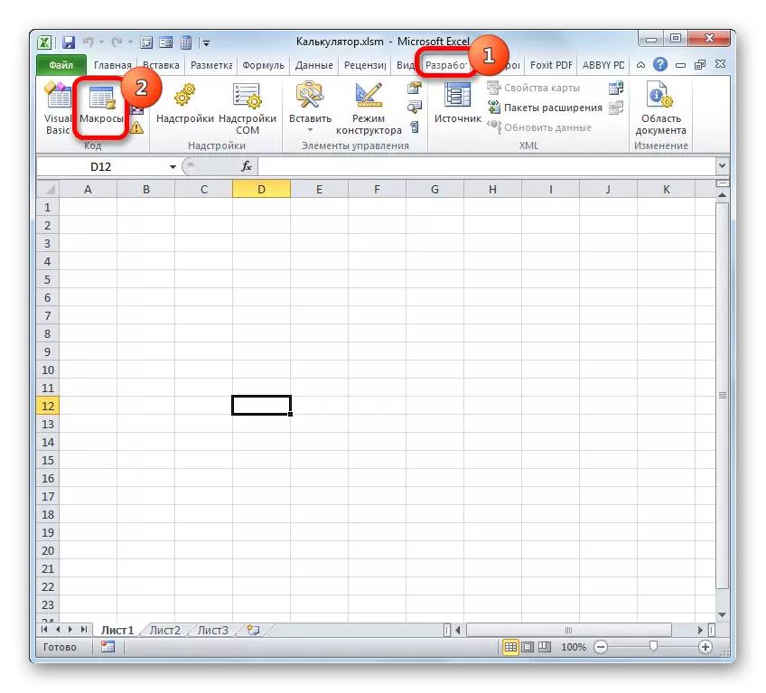
6. To start a computing tool using a macro while in the Developer tab, clay on the Macros icon on the tape in the "Code" tool block.



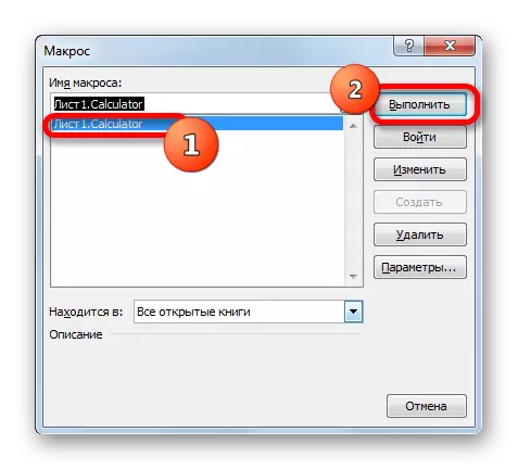
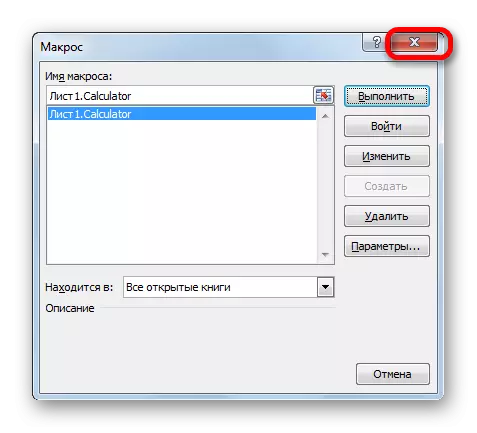
7. After that, the macro window starts. Choose the name of that macro, which we just created, allocate it and click on the "Run" button.



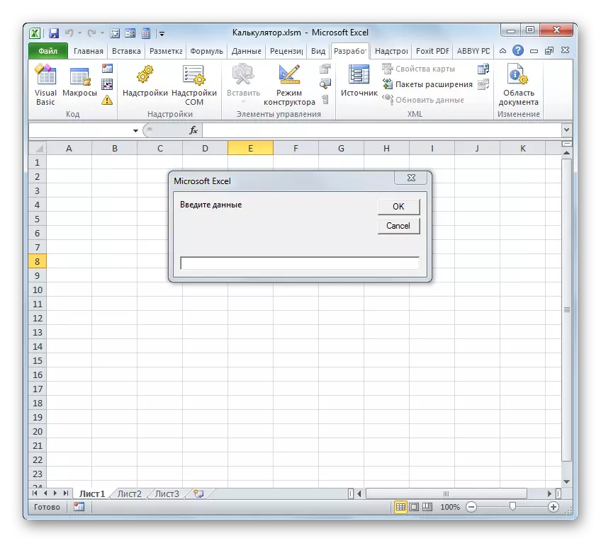
8. After performing this action, the calculator is launched based on the macro.



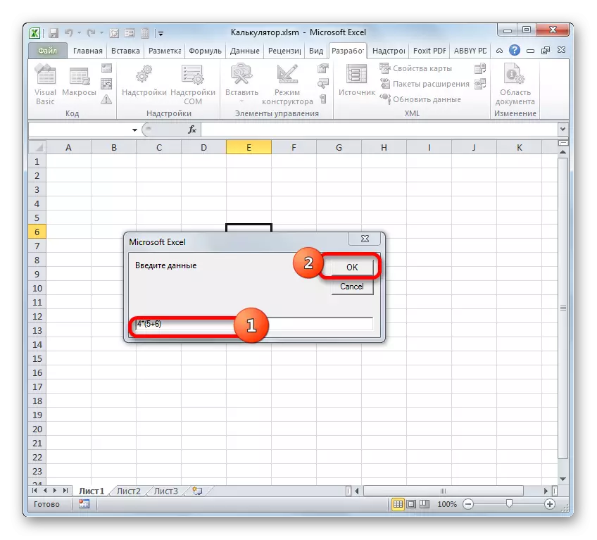
9. In order to make a calculation in it, write in the field the necessary action. The most convenient to use the numeric keyboard block for these purposes, which is located on the right. After the expression is entered, press the "OK" button.



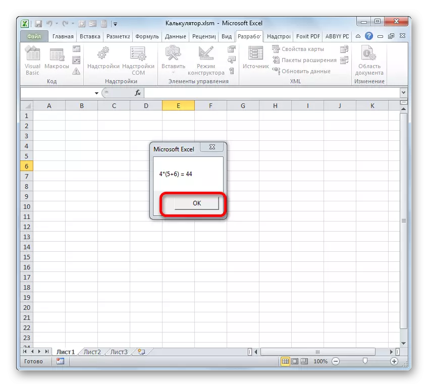
10. Then a small window appears on the screen, which contains the answer to the solution of the specified expression. To close it, press the "OK" button.



11. But agree that it is quite uncomfortable every time you need to make computing actions, switch to the macros window. Let's simplify the implementation of the launch of the calculation window. To do this, while in the Developer tab, click on the Macros icon already familiar to us.



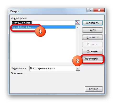
12. Then in the macros window, select the name of the desired object. Click on the "Parameters ..." button.



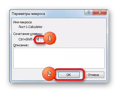
13. After that, the window is launched even less than the previous one. In it, we can set a combination of hot keys, when you click on which the calculator will be launched. It is important that this combination is not used to call other processes. Therefore, the first alphabet characters are not recommended. The first key of the combination sets the Excel program itself. This is the Ctrl key. The following key sets the user. Let it be the V key (although you can choose another). If this key is already used by the program, another key will automatically be added to the combination - SHIFT. We enter the selected symbol in the "Keyboard Combination" field and click on the "OK" button.



14. Then close the macro window by clicking on the standard closing icon in the upper right corner.

Now, when you set the selected combination of hot keys (in our case, CTRL + SHIFT + V) will start the Calculator window. Agree, it is much faster and easier than to call it every time through the macro window.

Lesson: How to create a macro in Excele

Method 2: Apply Functions

Now let's consider the option of creating a narrow-profile calculator. It will be designed to perform specific, specific tasks and is located directly on the Excel sheet. To create this tool, the built-in features of Excel will be applied.

For example, create a mass conversion tool. In the process of its creation, we will use the PREBO function. This operator relates to the engineering unit of the EXEL's built-in features. Its task is to transform the values ​​of one measurement measure to another. The syntax of this feature is as follows:

= Predoob (number; Ex_Dad_ism; Kon_d_ism)

"Number" is an argument that has a type of numerical value of the magnitude that must be converted to another measurement measurement.

"The initial unit of measure" is an argument that determines the unit of measurement value to be convened. It is defined by a special code that corresponds to a specific unit of measure.

"The final unit of measurement" is an argument that determines the unit of measurement of the magnitude into which the initial number is converted. It also specifies with the help of special codes.

We should stay in more detail on these codes, as they need them in the future when creating a calculator. Specifically, we need codes of units of mass measurement. Here are their list:

• G - gram;
• kg - kilogram;
• Mg - milligram;
• LBM - English pound;
• OZM - oz;
• SG - SALE;
• U is an atomic unit.

It is also necessary to say that all the arguments of this feature can be set as values ​​and links to the cells where they are placed.

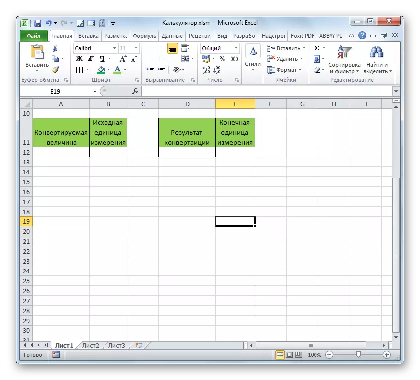
1. First of all, we make the workpiece. Our computing tool will have four fields:
   • Convertible value;
   • Source unit of measurement;
   • Result of conversion;
   • The final unit of measurement.

   We install headlines under which these fields will be placed and allocate their formatting (fill and borders) for more visual visualization.

   In the "Convertible value" field, the "source limit of measurement" and "final measurement limit" will be entered by data, and in the "Conversion Result" field - an end result is output.



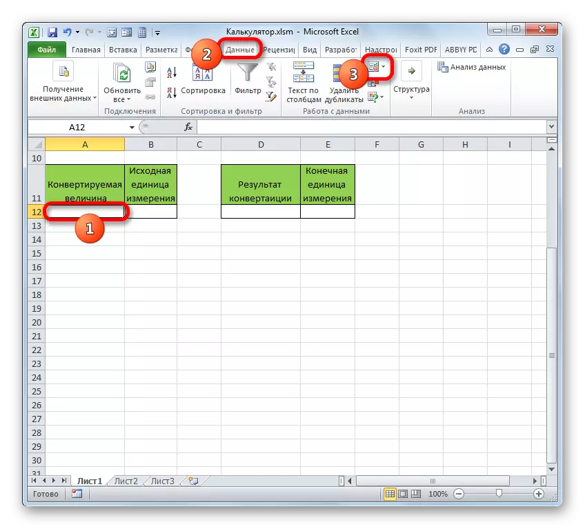
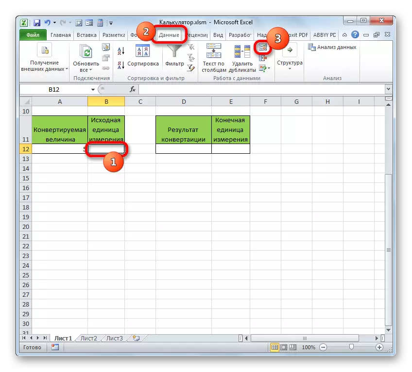
2. We do so that the user can enter only permissible values ​​in the "Convertible value" field, namely the numbers more zero. Select the cell into which the transformed value will be made. Go to the "Data" tab and in the "Working with Data" toolbar on the "Data Verification" icon.



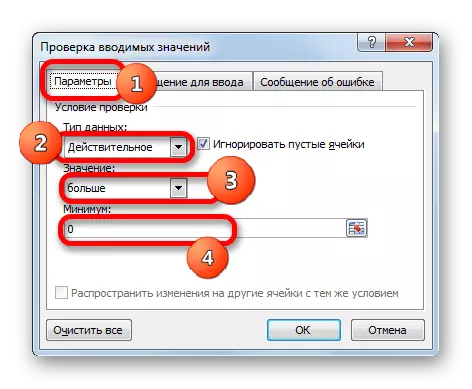
3. The "Data Verification" tool is launched. First of all, you will perform the settings in the "Parameters" tab. In the Data Type field, select the "Valid" parameter. In the "Value" field, also stop the choice on the "More" parameter. In the "Minimum" field, set the value "0". Thus, only valid numbers can be administered to this cell (including fractional), which are larger than zero.



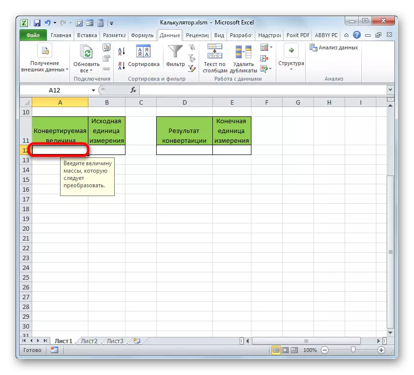
4. After that, we move to the tab of the same window "Message to Input" window. Here you can give an explanation that it is necessary to enter the user. It will see it when highlighting the cell input. In the "Message" field, write the following: "Enter the mass value that convert".



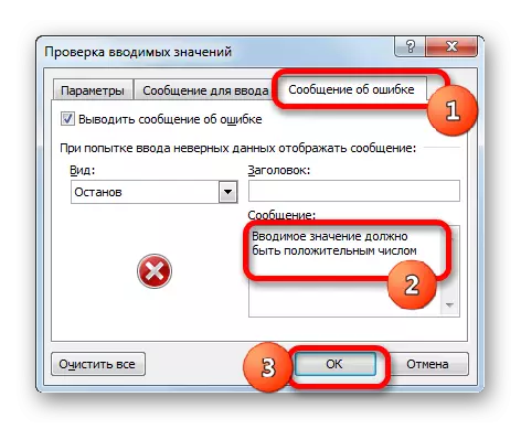
5. Then we move to the "Error Message" tab. In the "Message" field, we should write the recommendation that the user will see if incorrect data enters. Welcome the following: "The input value must be a positive number." After that, to complete the operation in the verification window of the input values ​​and save the settings entered by us, click on the "OK" button.



6. As we see, when the cell is selected, a hint for input appears.



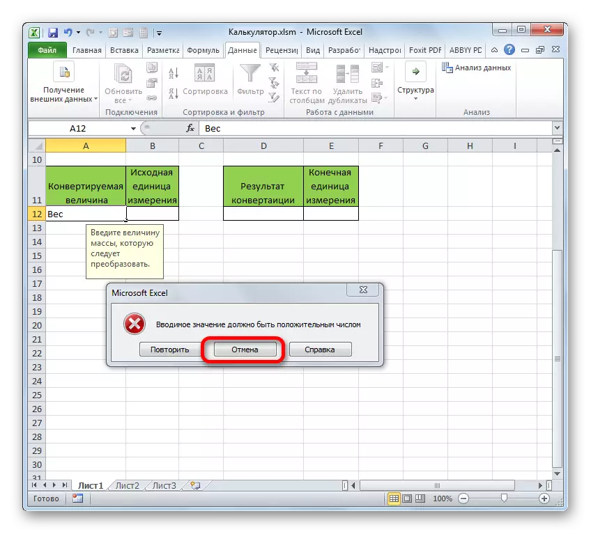
7. Let's try entering the incorrect value, for example, text or negative number. As you can see, an error message appears and the input is blocked. Click on the "Cancel" button.



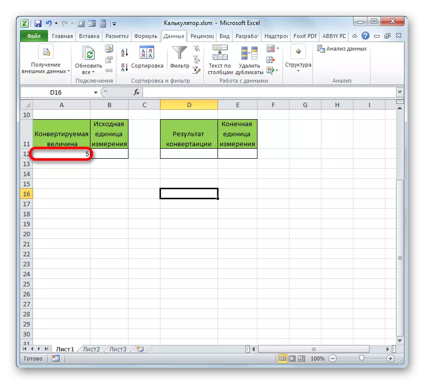
8. But the correct value is introduced without problems.



9. Now we go to the field "Source Unit of Measurement". Here we will do that the user will choose a value from the list consisting of those seven mass values, the list of which was given above when describing the arguments of the application function. Enter other values ​​will not work.

   We highlight the cell, which is under the name "Source Unit of Measurement". Again, clay on the "Data Check" icon.



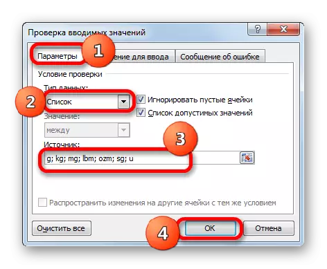
10. In the data verification window that opens, go to the "Parameters" tab. In the "Data Type" field, set the "List" parameter. In the field "Source" through a semicolon (;) we list the names of the mass of the mass for the pre-conversation function about which the conversation was higher. Next, click on the "OK" button.



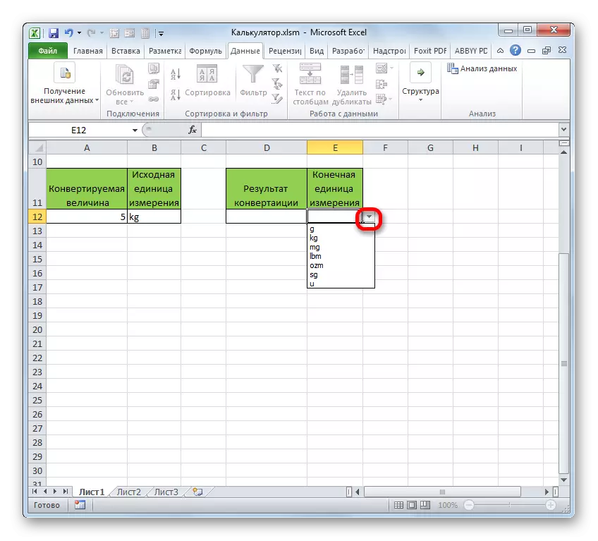
11. As you can see, now, if you select the field "Source Unit of Measurement", then a pictogram in the form of a triangle occurs to the right of it. When clicking on it opens a list with the names of the mass measurement units.



12. An absolutely similar procedure in the "Data Check" window is carried out with a cell with the name "Final Unit of Measurement". It also obtains exactly the same list of units of measurement.



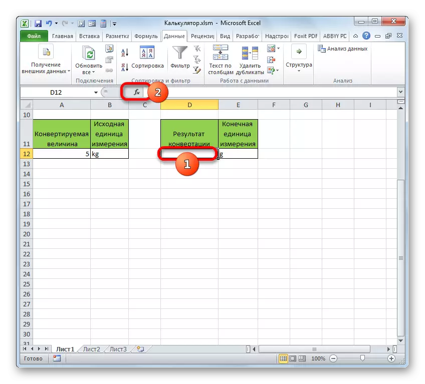
13. After that, go to the "conversion result". It is in it that will contain the function of the PRIOG and output the result of the calculation. We allocate this element of the sheet and click on the "Paste Function" icon.



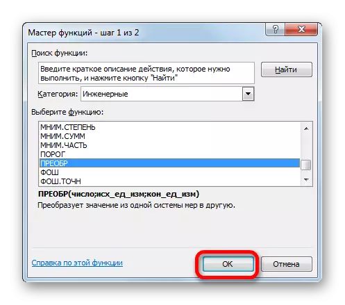
14. The functions master starts. Go to it in the category "Engineering" and allocate the name "Preobs" there. Then clay on the "OK" button.



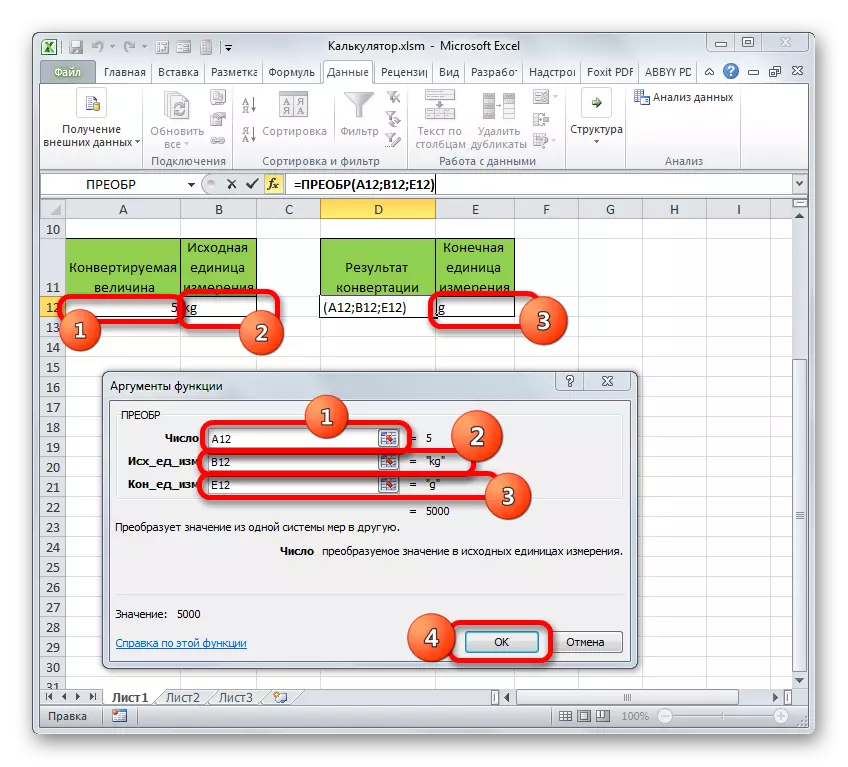
15. The opening window of the application operator's arguments occurs. In the "Number" field, it is necessary to enter the coordinates of the cell under the name "Convertible value". To do this, put it in the cursor in the field and click the left mouse button on this cell. Her address is immediately displayed in the field. In the same way, we introduce the coordinates in the field "Source Unit" and "Final Measurement Unit". Only this time by clicking on cells with the same names as these fields.

    After all the data is entered, press the "OK" button.



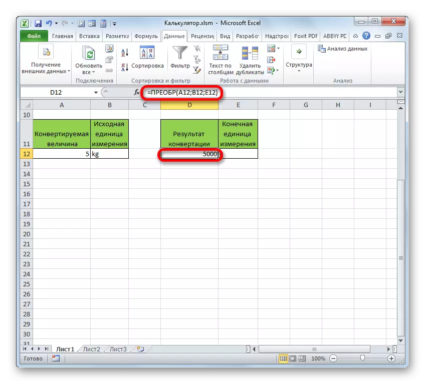
16. As soon as we completed the last action, in the cell "The result of conversion" there, the result of the magnitude conversion, according to the previously entered data, was immediately displayed.



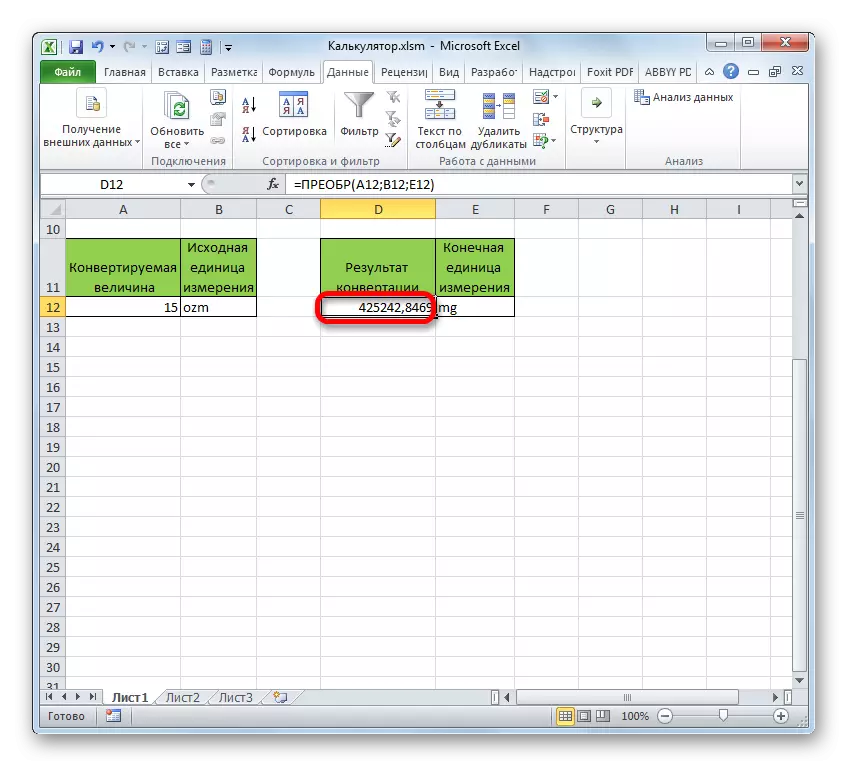
17. Let's change the data in the "Convertible value" cells, the "initial measurement unit" and "final unit of measure". As we see, the function when changing the parameters automatically recalculates the result. This suggests that our calculator fully functioning.



18. But we did not make one important thing. Cells for entering data are protected from introducing incorrect values, but the element for data output is not protected. But in general, it is impossible to enter anything at all, otherwise the calculation formula will simply be removed and the calculator will come into a non-working condition. By mistake in this cell you can enter the data and you yourself, not to mention third-party users. In this case will have to re-record the entire formula. You need to block any data entry here.

    The problem is that the blocking is installed on the sheet as a whole. But if we block the sheet, we will not be able to enter data in the input fields. Therefore, we will need in the properties of the cell format to remove the ability to lock from all elements of the sheet, then return this possibility only to the cell to output the result and then block the sheet.

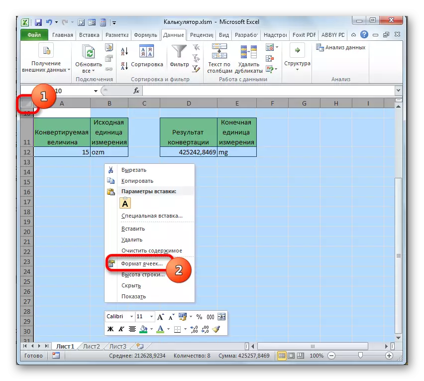
    Click on the left mouse button on the element at the intersection of the horizontal and vertical coordinate panel. This highlights the entire sheet. Then click right-click on the selection. A context menu opens, in which you select the position "cell format ...".



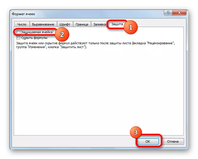
19. The formatting window is started. Go to the "Protection" tab in it and remove the checkbox from the "Protected Cell" parameter. Then clay on the "OK" button.



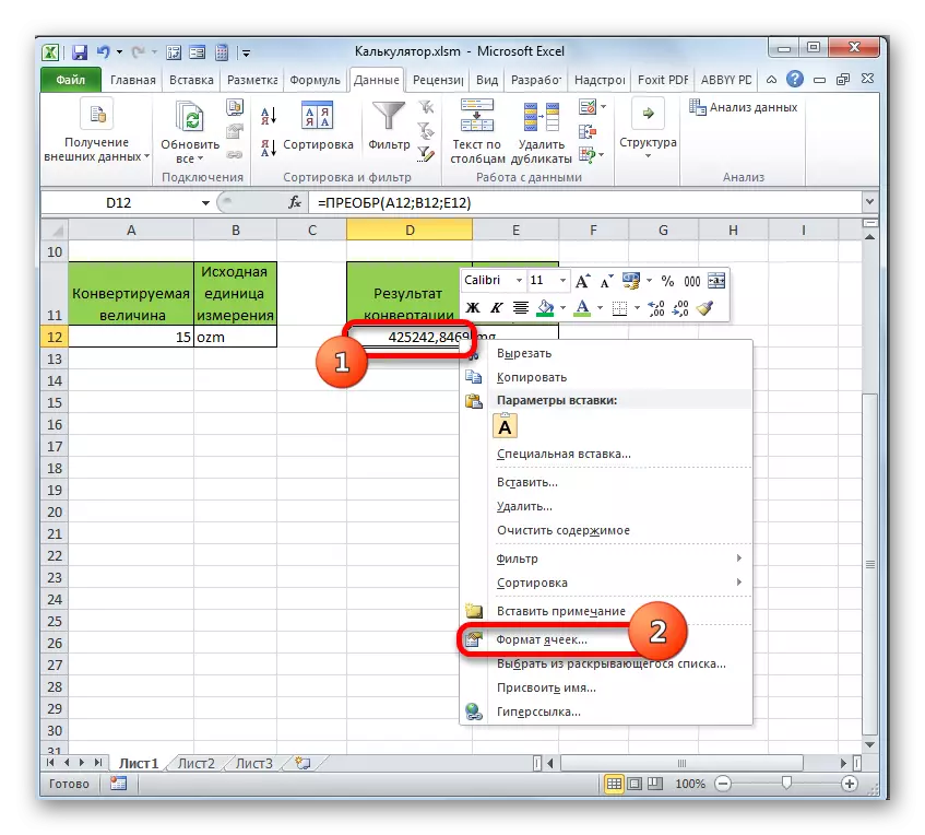
20. After that, we allocate only the cell to output the result and click on it right mouse button. In the context menu, clay on the "Format of the cells".



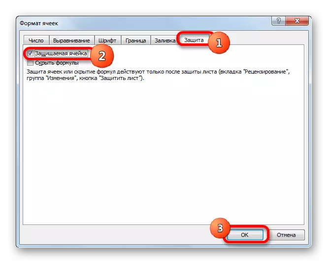
21. Again in the formatting window, go to the "Protection" tab, but this time, on the contrary, set the box near the "Protected Cell" parameter. Then click on the "OK" button.



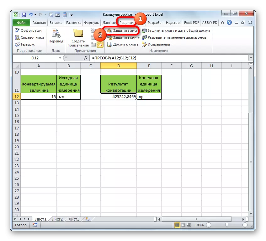
22. After that, we move to the "Review" tab and click on the "Protect Leaf" icon, which is located in the "Change tool" block.



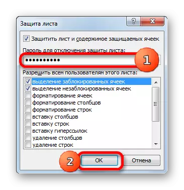
23. A sheet protection window opens. In the "Password to disable sheet protection", we enter a password, with which, if necessary, you can remove the protection in the future. The remaining settings can be left unchanged. Click on the "OK" button.



24. Then another small window opens, in which the password input should be repeated. We do it and click on the "OK" button.



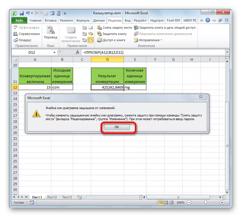
25. After that, when you try to make any changes to the output cell, the action result will be blocked, as reported in the emerging dialog box.

Thus, we have created a full-fledged calculator for converting the magnitude of the mass in different units of measurement.

In addition, in a separate article, it is described about the creation of another species of a narrow-profile calculator in Excele to calculate payments on loans.

Lesson: Calculation of annuity pay in Excel

Method 3: Enabling the Embedded Excel Calculator

In addition, exile has its own built-in universal calculator. True, by default, the launch button is missing on the tape or on the quick access panel. Consider how to activate it.

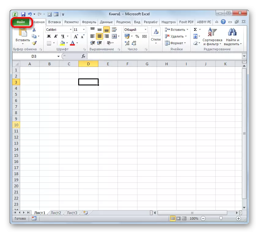
1. After starting the Excel program, we move to the "File" tab.



2. Next, in the window that opens, go to the "Parameters" section.



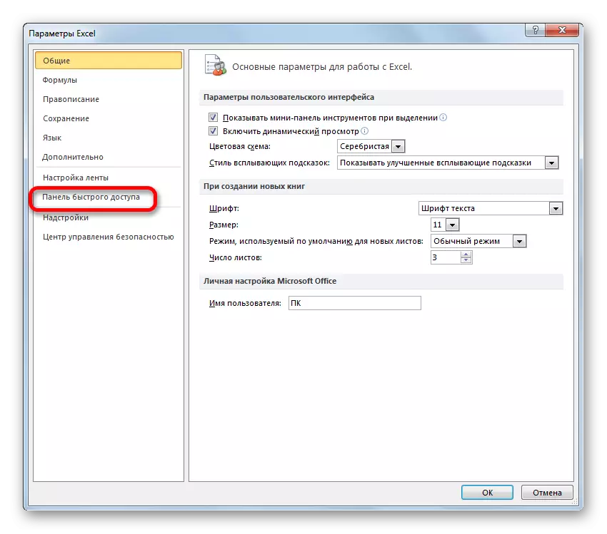
3. After starting the Excel parameters window, we move to the Fast Access Panel subsection.



4. The window opens, the right side of which is divided into two areas. In the right part it is located tools that have already been added to the shortcut panel. The left presents the entire set of tools that is available in Excel, including missing on the tape.

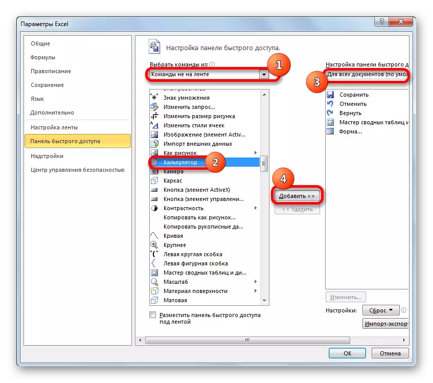
   Over the left area in the "Select Commands" field, select the "Commands not on the tape" field. After that, in the list of instruments of the left domain, looking for the name "Calculator". It will be easy to find, since all the names are alphabetically located. Then make the allocation of this name.

   Above the right area is the "Configuration of the Quick Access Panel". It has two parameters:

   • For all documents;
   • For this book.

   By default, configured for all documents. This parameter is recommended to be left unchanged if there are no prerequisites for the opposite.

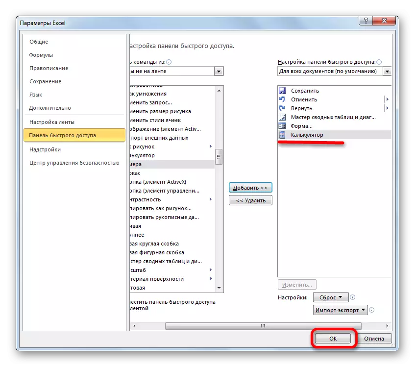
   After all settings are made and the name "Calculator" is highlighted, click on the "Add" button, which is located between the right and left domain.



5. After the name "Calculator" appears in the right window, press the "OK" button below.



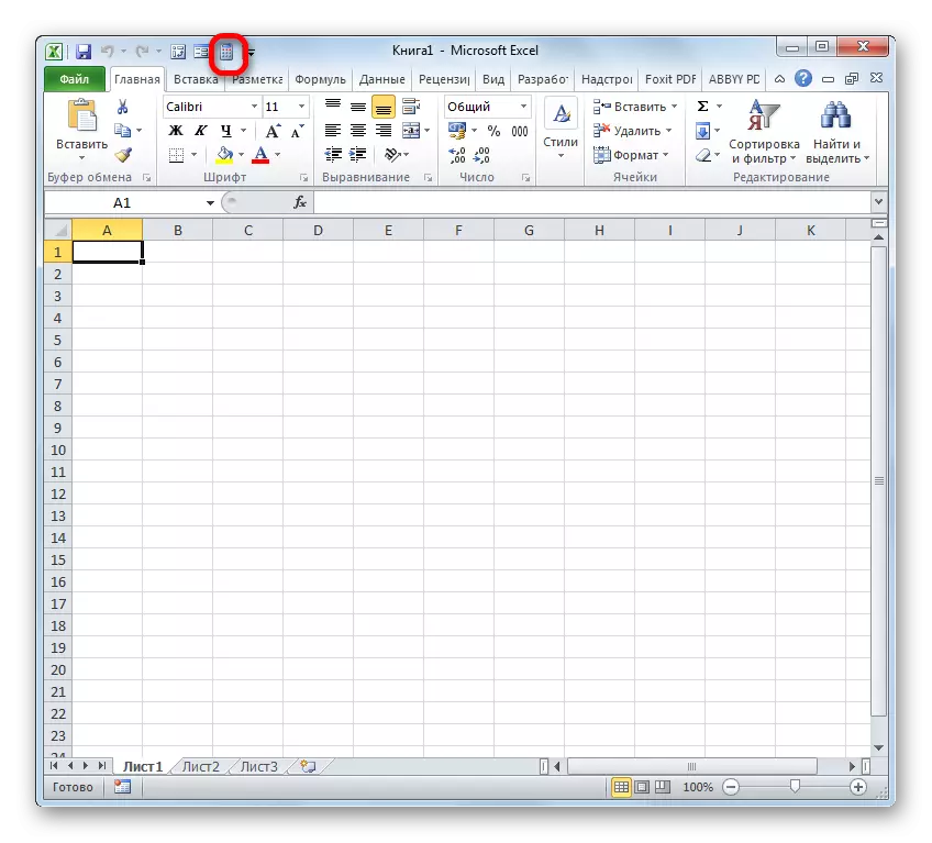
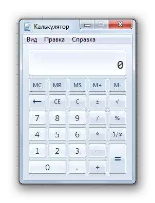
6. After this window, the Excel parameters will be closed. To start the calculator, you need to click on the icon of the same name, which is now located on the shortcut panel.



7. After that, the "Calculator" tool will be launched. It functions, as an ordinary physical analogue, only on the buttons you need to press the mouse cursor, its left-click.

As we see, there are a lot of options for creating calculators in Excele for various needs. This feature is especially useful when carrying out narrow-profile calculations. Well, for ordinary needs, you can use the built-in program tool.