Excel: Too many different cell formats

One of the problems with which users meet when working with tables in Microsoft Excel, is the error "Too many different cell formats". It is especially common when working with tables with XLS extension. Let's figure it out in the essence of this problem and find out what methods it can be eliminated.

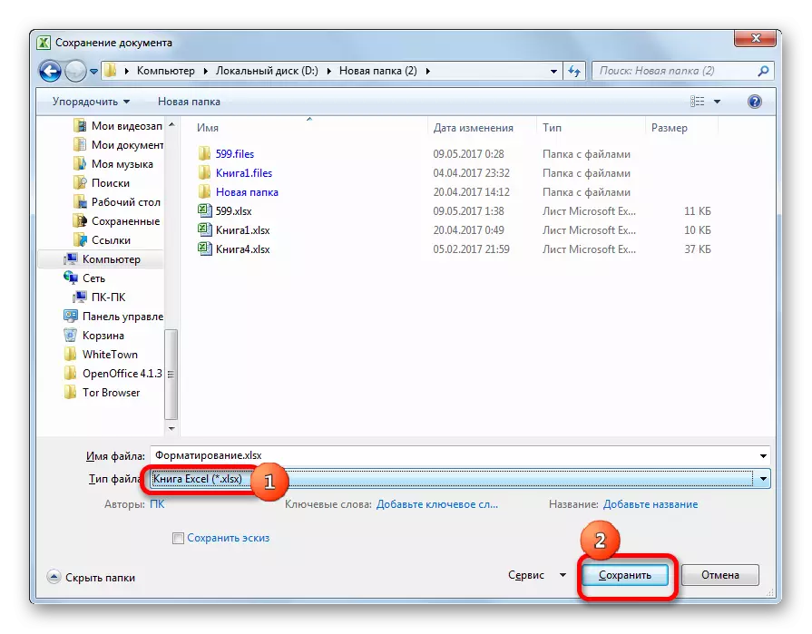
Now the document will be saved with the expansion of XLSX, which will allow you to work with a large amount of 16 times the number of formats simultaneously than it was when working with the XLS extension file. In the overwhelming majority of cases, this method allows to eliminate the error we studied.

Method 2: Cleaning formats in empty lines

But still there are cases when the user works precisely with the expansion of XLSX, but it still occurs this error. This is due to the fact that when working with the document, the frontier of 64,000 formats was exceeded. In addition, for certain reasons, a situation is possible when you need to save the file with the expansion of XLS, and not XLSX, since with the first, for example, can work more third-party programs. In these cases, you need to look for another way out of the current situation.

Often, many users format the place under the table with a margin so that in the future does not waste time on this procedure in the event of the table expansion. But this is an absolutely wrong approach. Because of this, the file size is significantly increased, work with it is slowed down, moreover, such actions may result in an error that we are discussing in this topic. Therefore, from such excesses should be rid of.

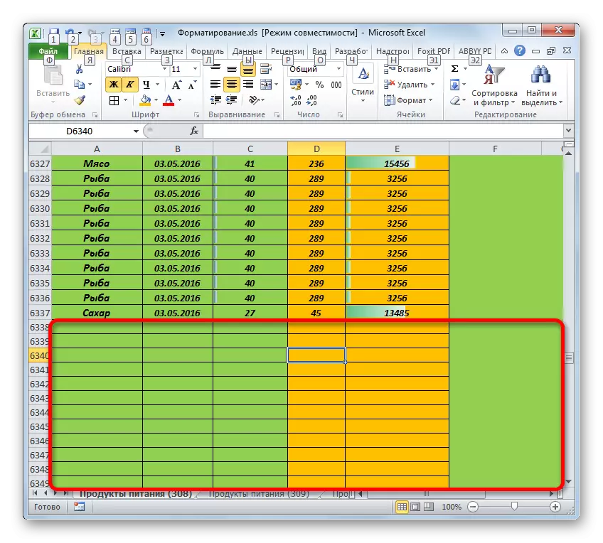
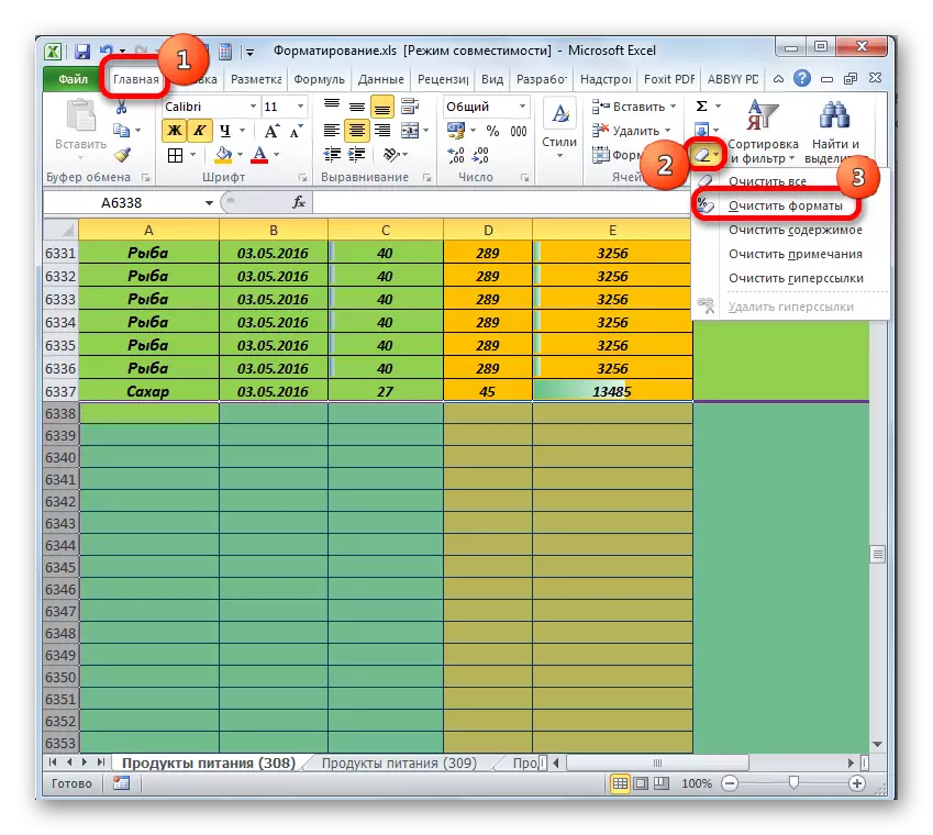
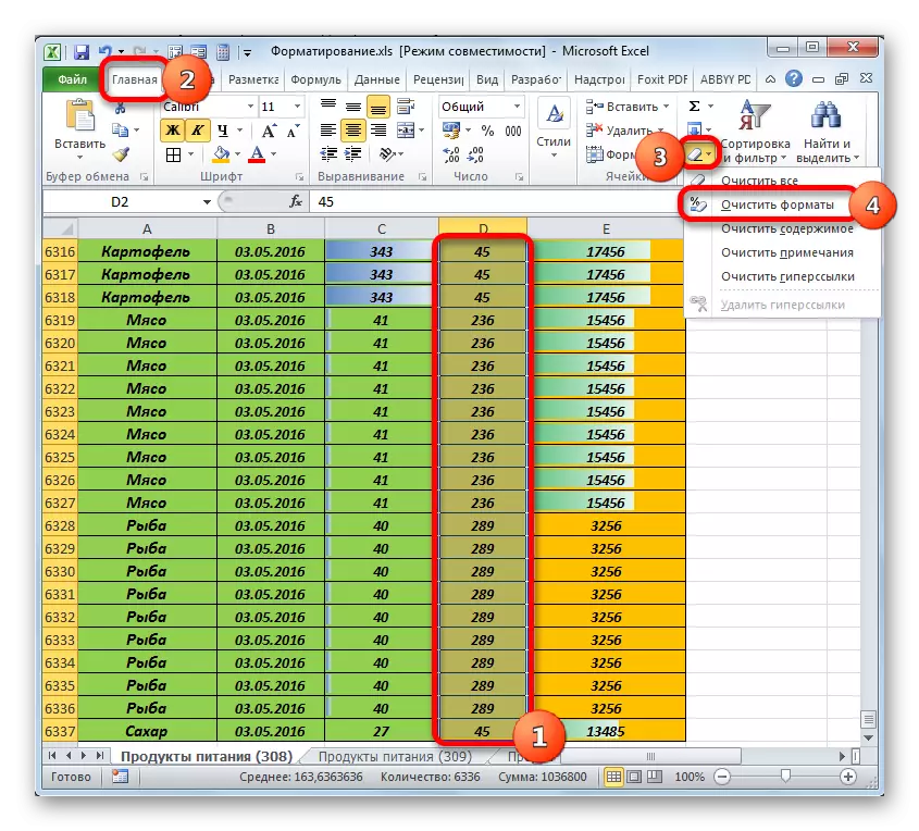
1. First of all, we need to highlight the entire area under the table, starting from the first string in which there is no data. To do this, click the left mouse button on the numeric name of this string on the vertical coordinate panel. Allocated to the entire line. Apply pressing the combination of the Ctrl + Shift button + down arrow down. Allocated the entire range of the document below the table.



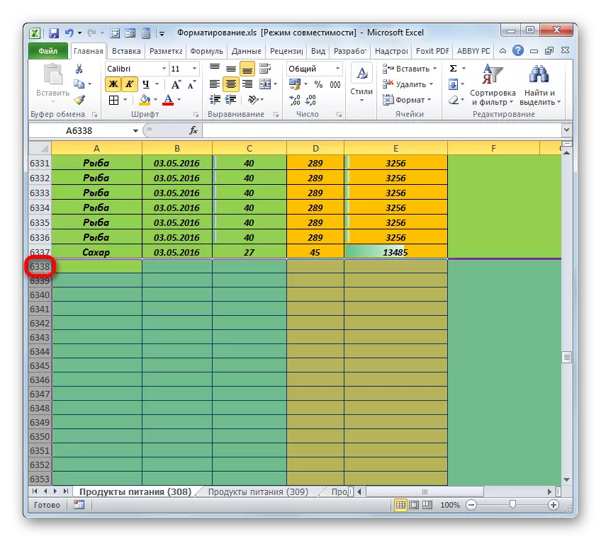
2. Then we move to the "Home" tab and click on the "Clear" tape icon, which is located in the Editing toolbar. A list opens in which you select the "Clear Formats" position.



3. After this action, the dedicated range will be cleaned.

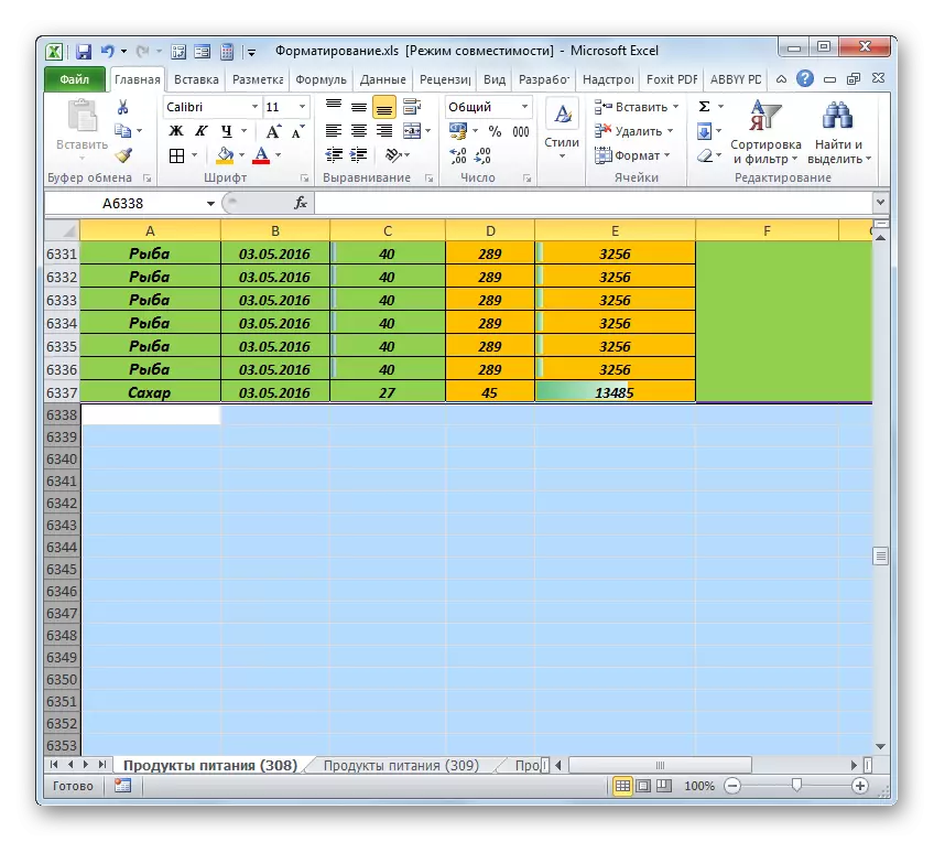
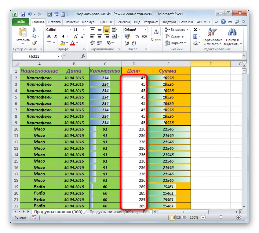
Similarly, it is possible to clean in the cells to the right of the table.

1. Clay on the name of the first not filled with the column in the coordinate panel. It is highlighted to the Niza himself. Then we produce a set of CTRL + SHIFT + arrow buttons to the right. This highlights the entire range of the document, located to the right of the table.



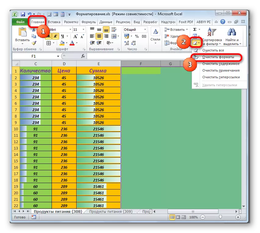
2. Then, as in the previous case, we click on the "Clear" icon, and in the drop-down menu, select the option "Clear Formats".



3. After that, cleaning will be cleaned in all cells to the right of the table.

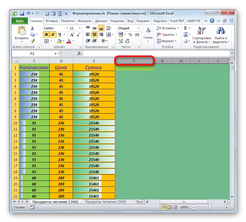
A similar procedure when an error occurs, we speak this lesson about this lesson, it will not be superfluous even if at first glance it seems that the bands below and the right of the table are generally not formatted at all. The fact is that they may have "hidden" formats. For example, text or numbers in a cell may not be, but it has a bold format in it, etc. Therefore, do not be lazy, in the event of an error, to carry out this procedure even over the outward empty bands. You also do not need to forget about possible hidden columns and lines.

Method 3: Deleting formats inside the table

If the previous version did not help solve the problem, then it is worth paying attention to excessive formatting within the table itself. Some users make formatting in the table even where it does not bear any additional information. They think that they make the table more beautiful, but in fact, quite often, such a design looks pretty tasteless. Even worse if the specified things lead to the braking of the program or an error that we describe. In this case, it should be left in the table only significant formatting.

1. In those ranges in which formatting can be removed completely, and this will not affect the informativeness of the table, we carry out the procedure according to the same algorithm, which was described in the previous method. First, we highlight the range in the table in which cleaning should be cleaned. If the table is very large, then this procedure will be more convenient to do, using the combinations of the Ctrl + Shift + arrow buttons to the right (left, up, down). If you select the cell inside the table, then using these keys, the selection will be made only inside it, and not until the end of the sheet, as in the previous method.

   We click on the already familiar to us "Clear" button in the Home tab. In the drop-down list, select the option "Clear Formats".



2. The highlighted range of the table will be completely cleaned.



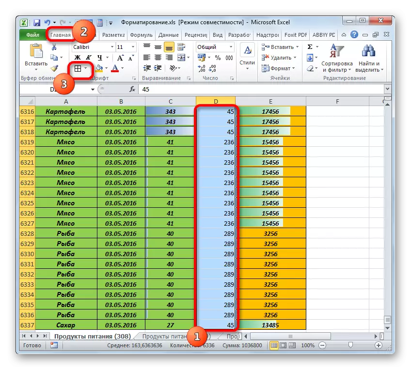
3. The only thing that needs to be done is to set the boundaries in the cleaned fragment if they are present in the rest of the table array.

But for some areas of the table, this option is not suitable. For example, in a specific range you can remove the fill, but the date format should be left, otherwise the data will be displayed incorrectly, boundaries and some other elements. The same version of the actions we talked about above, completely removes formatting.

But there is a way out and in this case, however, it is more laborious. In such circumstances, the user will have to allocate each block of homogeneously formatted cells and manually remove the format without which you can do.

Of course, it is a long and painstaking lesson, if the table is too big. Therefore, it is better right when drawing up a document not to abuse "beautiful" so that it does not have any problems that will have to spend a lot of time.

Method 4: Removal of conditional formatting

Conditional formatting is a very convenient data visualization tool, but its excessive application can also cause the error we studied. Therefore, you need to view the list of conditional formatting rules used on this sheet, and remove the position from it, without which you can do.

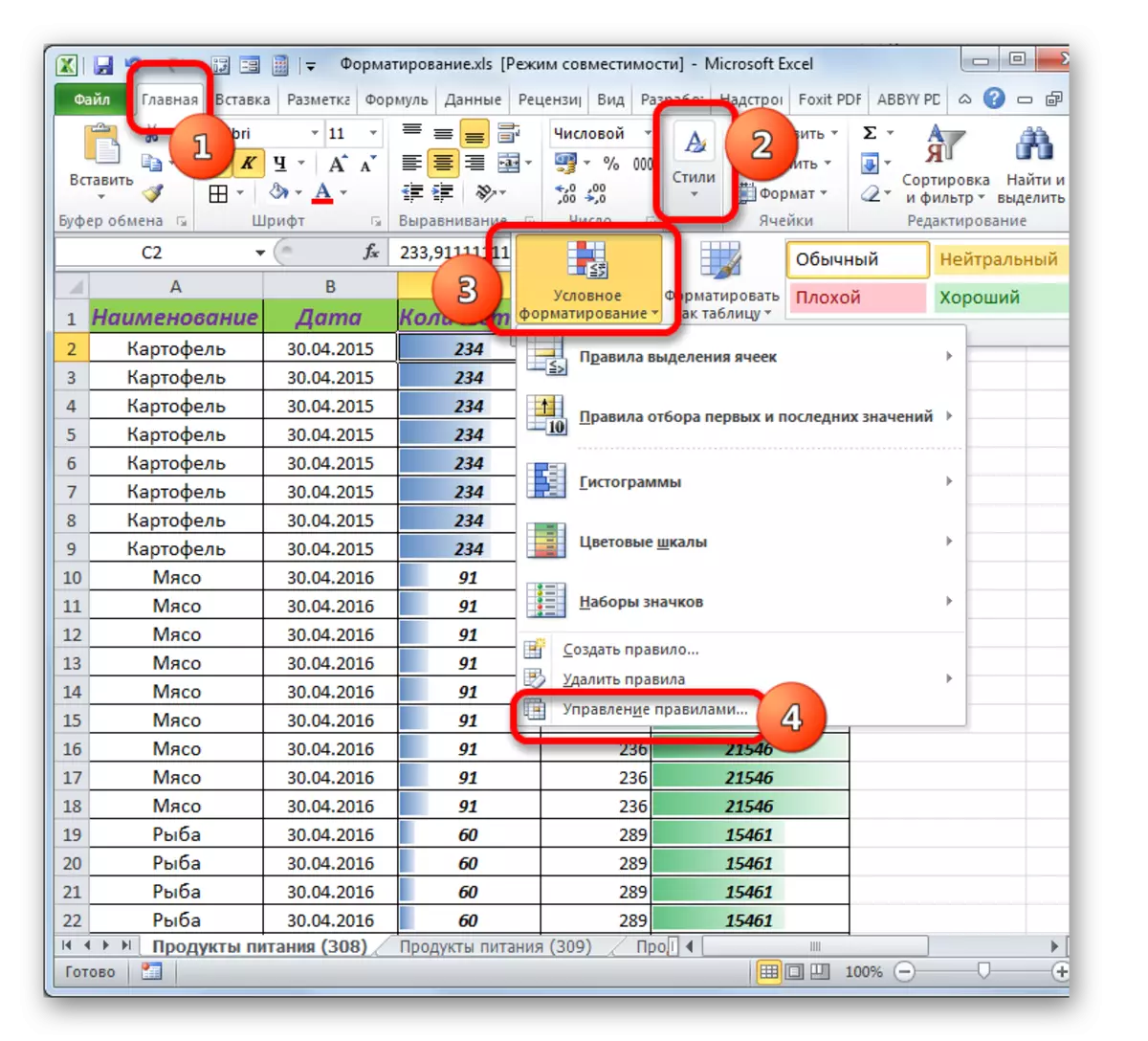
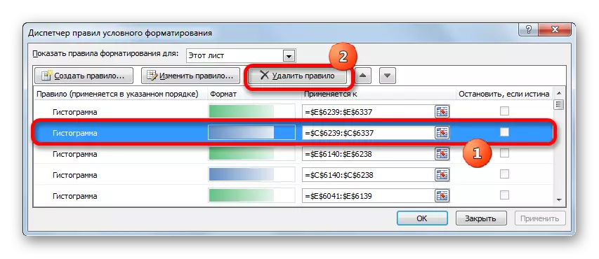
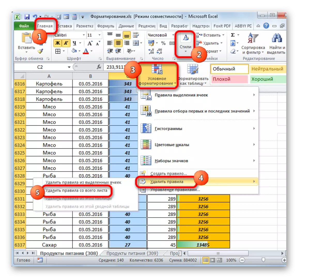
1. Located in the "Home" tab, clay on the "Conditional formatting" button, which is located in the "Styles" block. In the menu that will open after this action, select the "Management Rules" item.



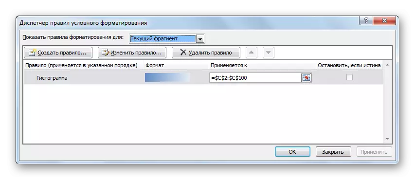
2. Following this, the rules management window is launched, which contains a list of conditional formatting elements.



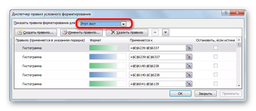
3. By default, only the elements of the selected fragment are located in the list. In order to display all the rules on the sheet, rearrange the switch in the "Show formatting rules for" the "This sheet" position. After that, all rules of the current sheet will be displayed.



4. Then we allocate the rule without which you can do, and click on the "Delete Rule" button.



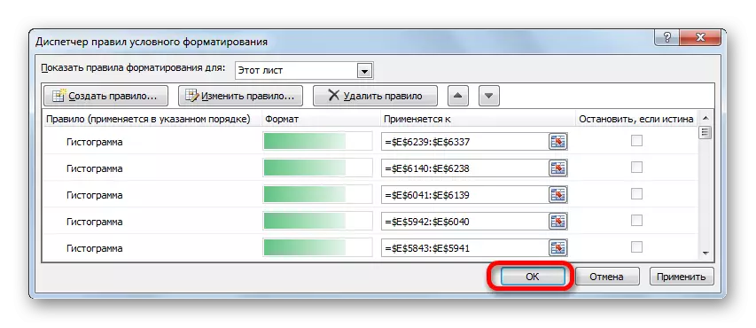
5. In this way, we remove those rules that do not play an important role in the visual perception of data. After the procedure is completed, press the "OK" button at the bottom of the rules manager window.

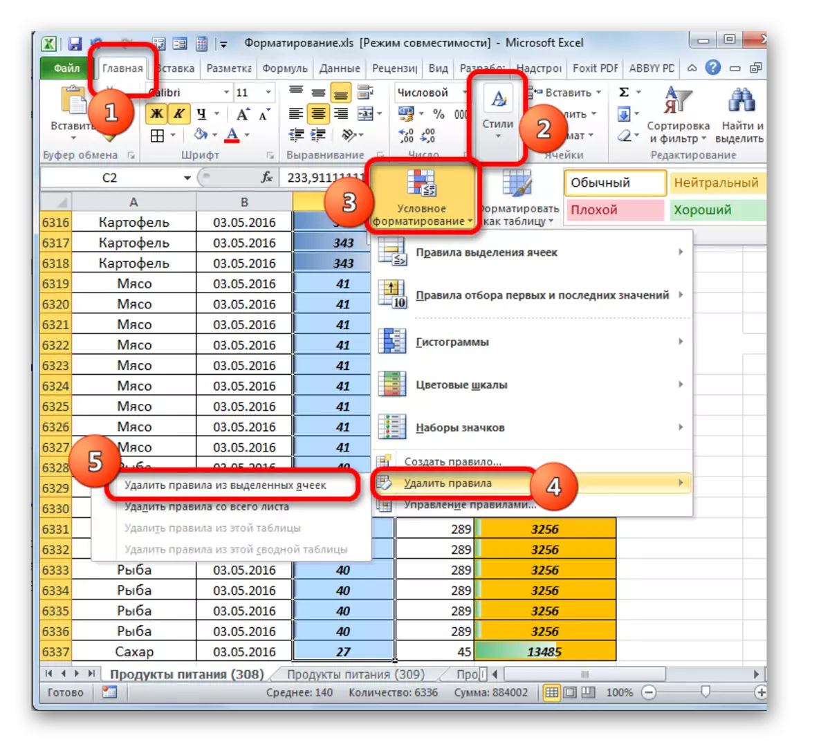
If you need to completely remove conditional formatting from a specific range, then it is even easier to do it.

1. We highlight the range of cells in which we plan to remove.



2. Click on the "Conditional Formatting" button in the "Styles" block in the Home tab. In the list that appears, select the "Delete Rules" option. Next, another list opens. In it, select "Delete rules from the selected cells".



3. After that, all rules in the dedicated range will be deleted.

If you want to completely remove conditional formatting, then in the last menu list you need to select the option "Delete rules from all over the sheet".

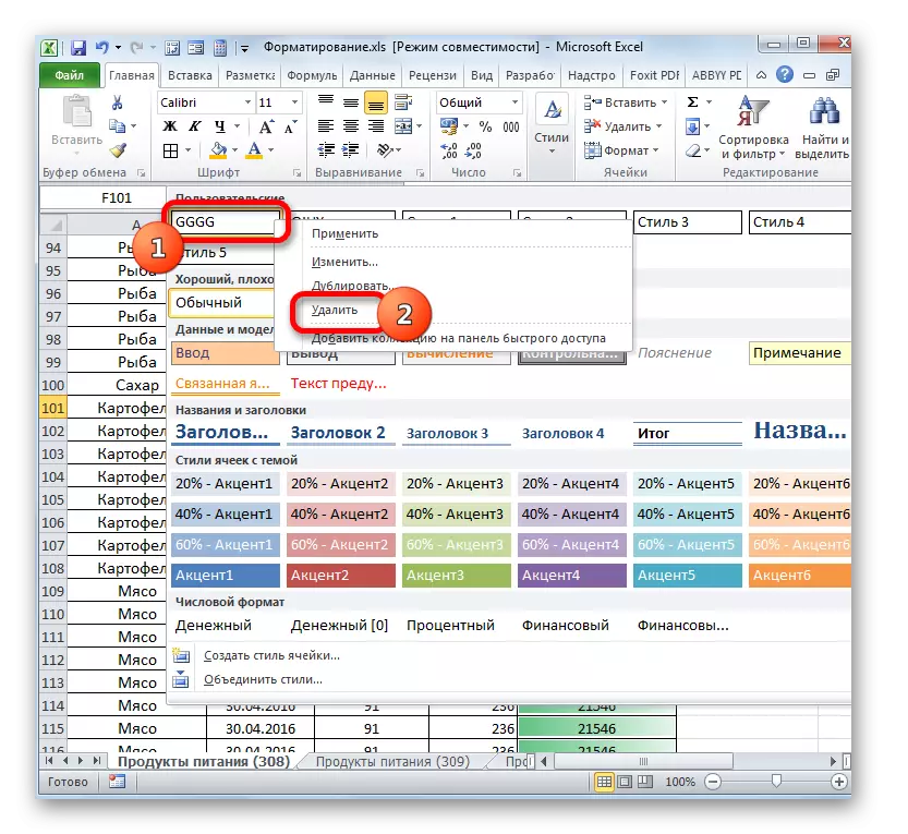
Method 5: Deleting custom styles

In addition, this problem may arise due to the use of a large number of custom styles. Moreover, they may appear as the result of import or copy from other books.

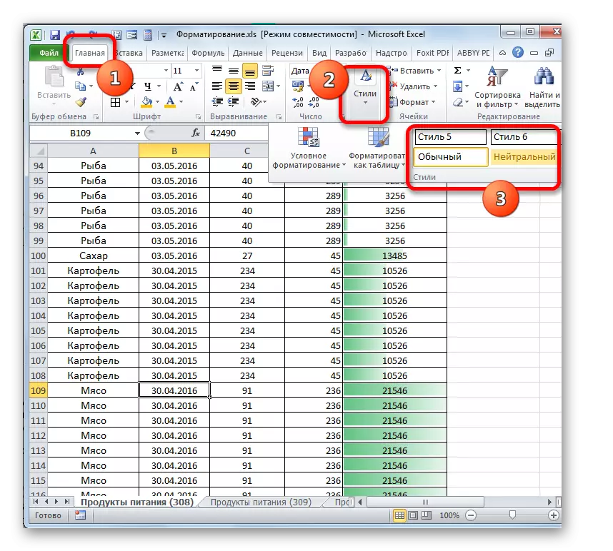
1. This problem is eliminated as follows. Go to the "Home" tab. On the tape in the "Styles" tools block click on the group "Styles of cells".



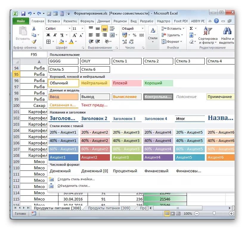
2. Opens the style menu. There are various styles of designs of cells, that is, in fact, fixed combinations of several formats. At the very top of the list there is a "Custom" block. Just these styles are not originally built into Excel, but are a product actions product. If an error occurs, the elimination of which we study are recommended to delete them.



3. The problem is that there is no built-in tool for mass removal of styles, so everyone will have to delete separately. We bring the cursor to a specific style from the "Custom" group. I click on it with the right mouse button and in the context menu, select the option "Delete ...".



4. We delete in this way each style from the "Custom" block until only the built-in Excel styles will remain.

Method 6: Deleting custom formats

A very similar procedure for removing styles is to delete custom formats. That is, we will delete those elements that are not built-in default in Excel, but implemented by the user, or were built into the document in another way.

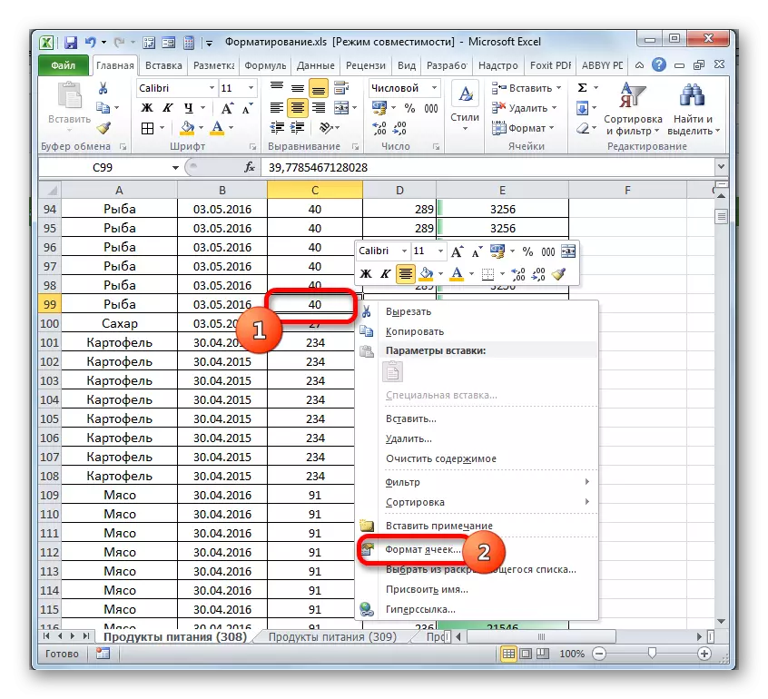
1. First of all, we will need to open the formatting window. The most common way to do is to click right-click on any place in the document and from the context menu to select the option "Cell format ...".

   

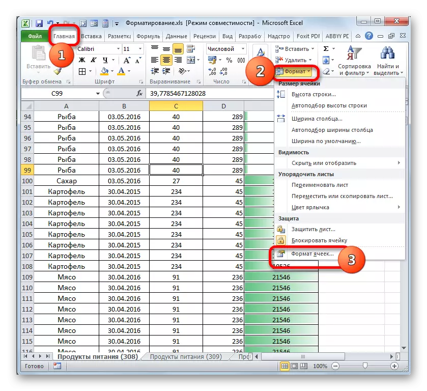
   You can also, while in the "Home" tab, click on the "Format" button in the "Cell" block on the tape. In the running menu, select the item "Format cells ...".

   

   Another option to call the window you need is a set of Ctrl + 1 keys on the keyboard.

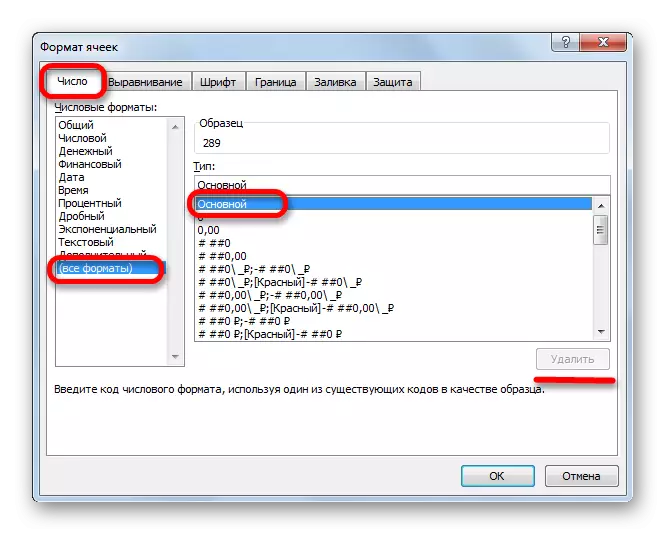
2. After performing any of the actions that were described above, the formatting window will start. Go to the "Number" tab. In the "Numeric Formats" parameters, we install the switch to the position "(all formats)". On the right side of this window, the field is located in which there is a list of all types of items used in this document.

   We highlight the cursor each one. Go to the next name more convenient with the "Down" key on the keyboard in the navigation unit. If the element is built-in, then the "Delete" button will be inactive.



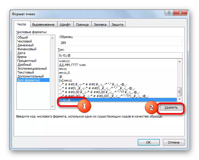
3. As soon as the added user element is highlighted, the "Delete" button will become active. Click on it. In the same way, delete all the names of custom formatting in the list.



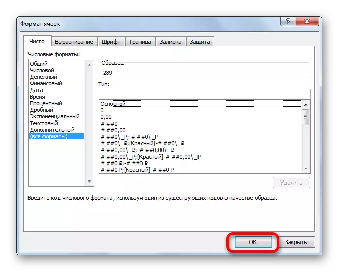
4. After completing the procedure, we must press the "OK" button at the bottom of the window.

Method 7: Removing unnecessary sheets

We described the action to solve the problem only within one sheet. But do not forget that exactly the same manipulations need to be done with all the other book filled with these sheets.

In addition, unnecessary sheets or sheets, where information is duplicated, it is better to delete at all. It is done quite simple.

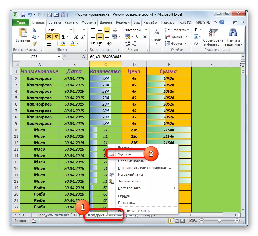
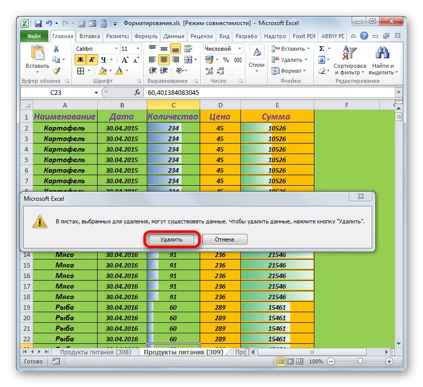
1. By clicking the right mouse button on the sheet shortcut, which should be removed above the status bar. Next, in the menu that appears, select "Delete ...".



2. After that, a dialog box opens that requires a confirmation of a shortcut removal. Click in it on the "Delete" button.



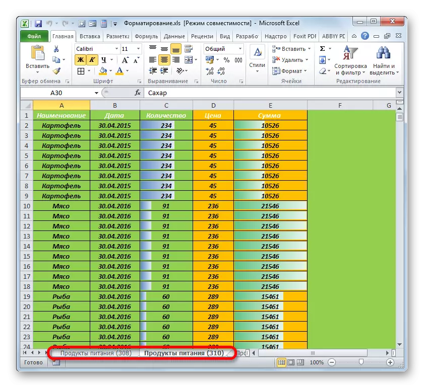
3. Following this, the selected label will be removed from the document, and, therefore, all the formatting elements on it.

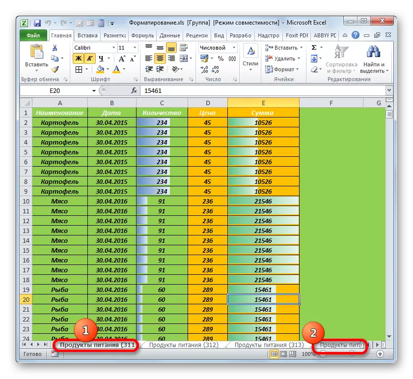
If you need to remove several sequentially located shortcuts, then click on the first of them with the left mouse button, and then click on the last one, but only at the same time holding the Shift key. All labels located between these elements will be highlighted. Next, the removal procedure is carried out on the same algorithm that was described above.

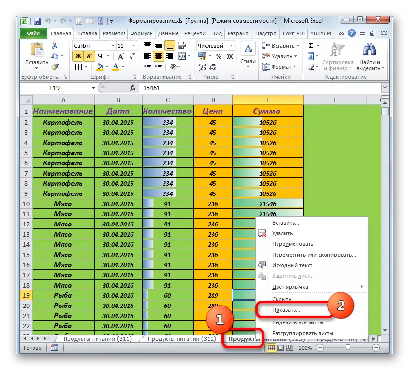
But there are also hidden sheets, and it can be quite a large number of different formatted elements. To remove excessive formatting on these sheets or delete them at all, you need to immediately display labels.

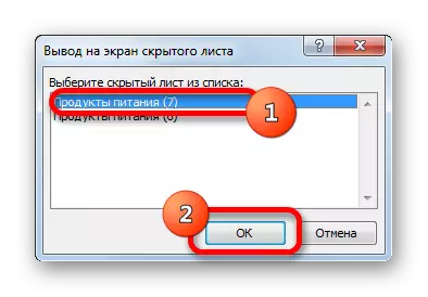
1. Click on any label and in the context menu, select the "Show" item.



2. A list of hidden sheets opens. Select the name of the hidden sheet and click on the "OK" button. After that, it will be displayed on the panel.

Such an operation is done with all the hidden sheets. Then we look at what to do with them: to completely remove or clean from redundant formatting if the information is important on them.

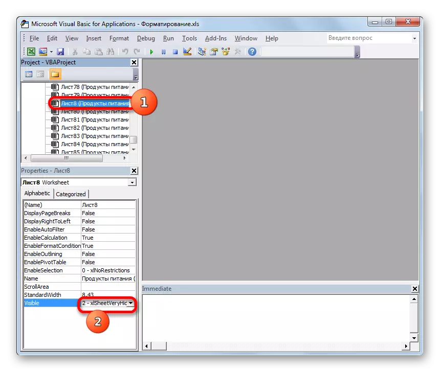
But besides this, there are also the so-called super-walled sheets, which in the list of ordinary hidden sheets you do not find it. They can be seen and displayed on the panel only through the VBA editor.

1. To start the VBA editor (macro editor), click the combination of hot keys Alt + F11. In the "Project" block, we allocate the name of the sheet. Here they are displayed as ordinary visible sheets, so hidden and superbry. In the bottom area "Properties" we look at the value of the "Visible" parameter. If there is set to "2-XLSheetVeryHidden", then this is a super-free sheet.



2. Click on this parameter and in the list that opens, select the name "-1-xlsheetvisible". Then click according to the standard closing button.

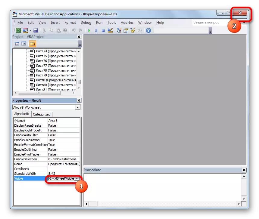
After this action, the selected sheet will stop being superbned and the label will be displayed on the panel. Next, it will be possible to conduct either the cleaning procedure or deletion.

Lesson: What to do if sheets are missing in Excel

As you can see, the fastest and efficient method will get rid of the error studied in this lesson - it is to save the file again with the XLSX expansion. But if this option does not work or for some reason it is not suitable, then the remaining ways to solve the problem will require a lot of time and effort from the user. In addition, all of them will have to be used in the complex. Therefore, it is better in the process of creating a document not to abuse redundant formatting so that then it does not have to spend the forces to eliminate the error.