Network graph in Excel

Network graph is a table designed to prepare a project plan and control over its implementation. For its professional construction there are specialized applications, such as MS Project. But for small businesses and especially personal economic needs, it makes no sense to buy specialized software and spend a sea of ​​time to teach the intricacies of work in it. With the construction of a network graph, the Excel table processor is completely successfully coped, which is installed from most users. Let's find out how to fulfill the above task in this program.

On this, the creation of a table of table can be considered finished.

Lesson: Formatting Tables in Excel

Stage 2: Creating a time scale

Now you need to create a bulk part of our network graphics - time scale. It will be a set of columns, each of which corresponds to one project period. Most often, one period is equal to one day, but there are cases when the amount of the period is calculated in weeks, months, quarters, and even years.

In our example, use the option when one period is equal to one day. Let's make a time scale for 30 days.

1. Go to the right border of the workpiece of our table. Starting from this boundary, we allocate a range of 30 columns, and the number of lines will be equal to the number of lines in the workpiece that we created earlier.



2. After that, clay on the "Border" icon in "All borders" mode.



3. Following the boundaries outlined, we will make dates in the time scale. Suppose we will control the project with a period of action from 1 to 30 June 2017. In this case, the name of the time scale column needs to be set according to the specified period of time. Of course, you manually fit all the dates rather tiring, so we use the tool for the autocillion, which is called "Progression".

   In the first object of the Time Shakal Hat insert the date "01.06.2017". Moving to the "Home" tab and clay on the "Fill" icon. An additional menu opens where you need to choose the item "Progression ...".



4. The activation of the "Progression" window is activated. The "Location" group must be marked the "on strings", since we will fill in the header represented as a string. In the Type group, the Date parameter must be marked. In the block "Units", put the switch near the position "Day". In the "Step" area there should be a digital expression "1". In the limit value, we indicate the date 06/30/2017. Click on "OK".



5. The array of caps will be filled with sequential dates in the limit of October 1 to June 30, 2017. But for the network schedule, we have too wide cells, which negatively affects the compactness of the table, and, it means, and on its visibility. Therefore, we will conduct a number of manipulations to optimize the table.

   Select the cap of the time scale. Clay on the dedicated fragment. The list is stopped at the Cell Format Point.



6. In the formatting window that opens, we move to the "Alignment" section. In the "Orientation" area, we set the value "90 degrees", or by moving the cursor the element "Inscription" up. Clay on the "OK" button.



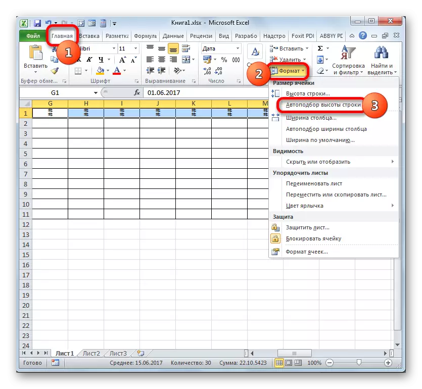
7. After this name, columns in the form of dates changed their orientation with horizontal to vertical. But due to the fact that the cells did not change their size, the names became unreadable, since they did not fit into the designated sheet elements by vertical. To change this position of things, allocate the contents of the header. Clay on the "Format" icon, located in the "Cell" block. In the list, you stop on the option "Auto-section of the height of the string."



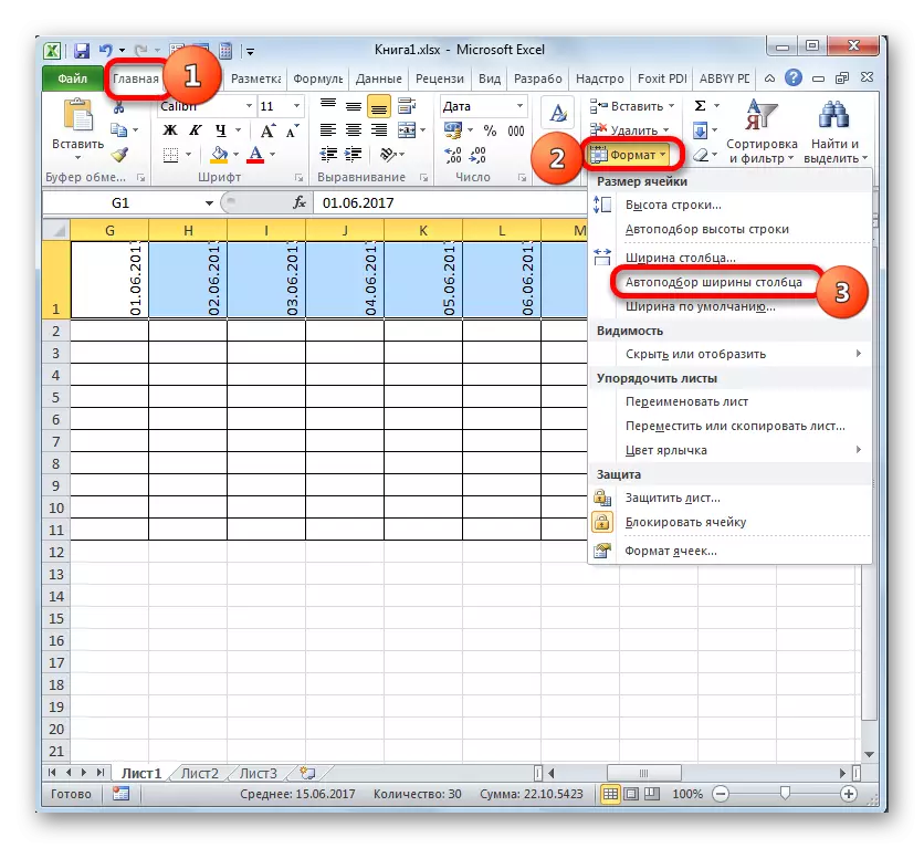
8. After the described action of the name of columns in height fit into the boundaries of the cells, but in the width of the cells did not become more compact. Again, we highlight the range of time caps and clay on the "Format" button. This time, in the list, select the option "Auto Column Width".



9. Now the table has acquired compactness, and the grid elements accepted the square shape.

Stage 3: Filling data

Next you need to fill out a data table.

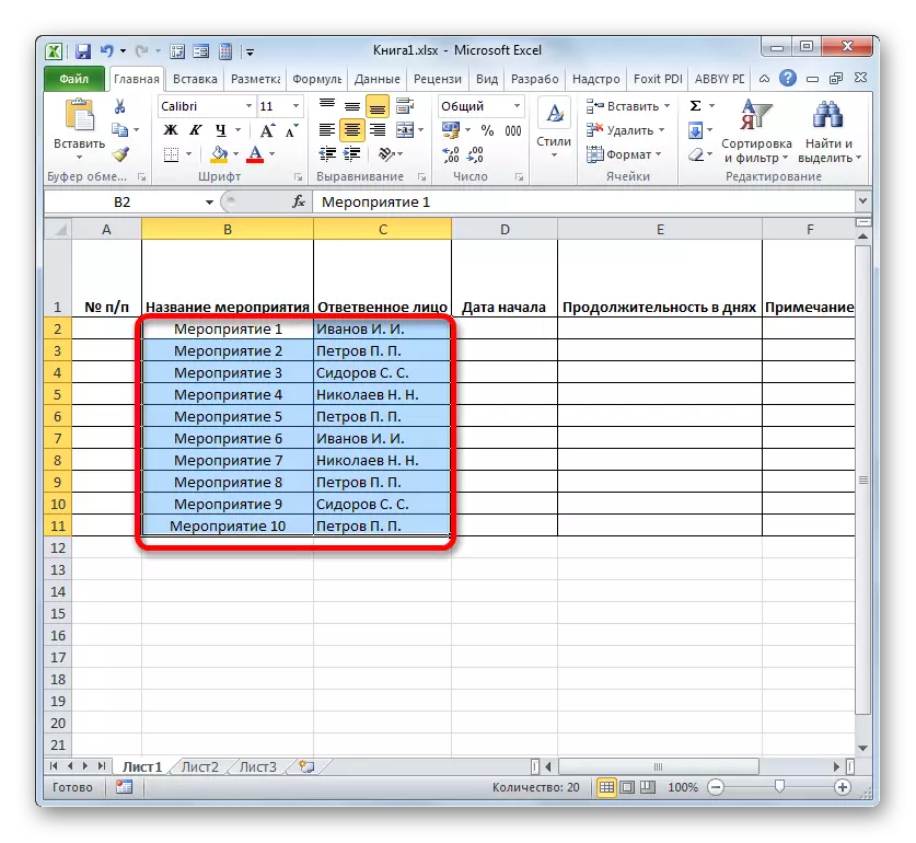
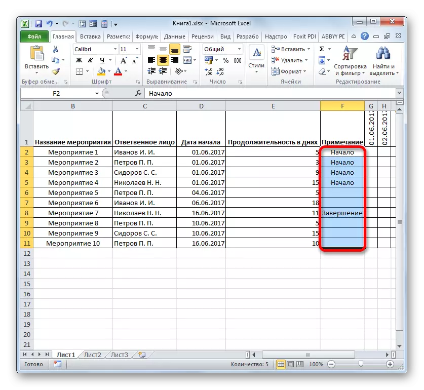
1. We return to the top of the table and fill in the "event name" column with the names of the tasks that are planned during the project. And in the next column, we introduce the names of responsible persons who will be responsible for fulfilling work on a specific event.



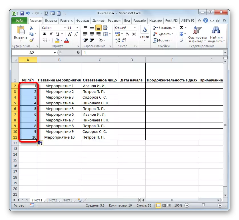
2. After that, you should fill in the "P / P" column. If the events are a bit, then this can be done, manually driven by the number. But if it is planned to perform many tasks, it will be more rational to resort to autofilement. To do this, we put in the first element of the column number "1". The cursor is directed to the lower right edge of the element, waiting for the moment when it is transformed into a cross. You simultaneously clamp the Ctrl key and the left mouse button, pull the cross down to the bottom limit of the table.



3. The entire column will be filled with values ​​in order.



4. Next, go to the "start date" column. Here you should specify the start date of each specific event. We do it. In the "Duration in the Days", we specify the number of days that will have to spend to solve the specified task.



5. In the "Notes" column, you can fill out data as needed, indicating the features of a specific task. Making information in this column is not mandatory for all activities.



6. Then we highlight all the cells of our table, except for the header and the grid with dates. Clay on the "Format" icon on the tape, to which we have previously addressed, we click in the list of the list of the column width "that opens.



7. After this, the width of the columns of the selected elements is narrowed to the size of the cell, in which the length of the data is most compared to the remaining elements of the column. Thus, the place is saved on the sheet. At the same time, in the table header, the names are transferred according to words in those elements of the sheet in which they do not fit into width. It turned out to be done due to the fact that we previously set the caps of the caps of the caps near the "Transfer according to" parameter.

Stage 4: Conditional Formatting

At the next stage of working with the network schedule, we will have to pour the color of the grid cell that correspond to the period of performing a specific event. This can be done by means of conditional formatting.

1. We mark the entire array of empty cells on the time scale, which is represented as a mesh of square shape elements.



2. Click on the "Conditional Formatting" icon. It is located in the "Styles" block then the list opens. It should choose the option "Create Rule".



3. The window is launched in which you want to form a rule. In the field of type selection, we note the item that implies the use of the formula to designate formatted elements. In the "Format Values" field, we need to set the release rule represented as a formula. For a specifically of our case, it will have the following form:

   = And (G $ 1> = $ d2; G $ 1

   But in order for you to convert this formula and for your network schedule, which is quite possible, will have other coordinates, we should decipher the recorded formula.

   "And" is the embedded Excel function, which checks whether all the values ​​made as its arguments are the truth. The syntax is:

   = And (logical_dation1; logical_dation2; ...)

   In total, up to 255 logical values ​​are used in the form of arguments, but we need only two.

   The first argument is recorded as an expression "G $ 1> = $ d2". It checks that the value in the time scale has more or equal to the corresponding date of the start of a certain event. Accordingly, the first link in this expression refers to the first cell of the string on the time scale, and the second is the first element of the column of the start date of the event. The dollar sign ($) is set specifically that the coordinates of the formulas in which this symbol is not changed, and remained absolute. And for your occasion, you must set the dollar icons in the appropriate places.

   The second argument is represented by the expression "G $ 1

   If both arguments of the formula represented will be true, then to cells, conditional formatting in the form of their fill with color will be applied.

   To select a certain color of the fill, clay on the "Format ..." button.



4. In a new window, moving to the "Fill" section. The group "Background colors" presents various types of disease. We note the color that the cells of the days corresponding to the period of performing a particular task are distinguished. For example, choose a green color. After the shade was reflected in the "Sample" field, clay on "OK".



5. After returning to the creation window, the rules also clay on the "OK" button.



6. After completing the last action, the array of the network graphic grid, corresponding to the period of execution of a particular event, were painted in green.

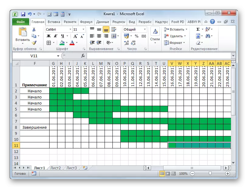
On this, the creation of a network graphics can be considered finished.

Lesson: Conditional formatting in Microsoft Excel

In the process of work, we have created a network schedule. This is not the only option of a similar table that can be created in Excele, but the basic principles of performing this task remain unchanged. Therefore, if desired, each user can improve the table represented in the example under its specific needs.